Automation System Engineer
Basics of Relays, Contactor, MCB, MCCB, ELCB, RCD, ACB
Relays:
A relay is an electrically operated switch. Many relays use an electromagnet to operate a switching mechanism mechanically, but other operating principles are also used. Relays are used where it is necessary to control a circuit by a low-power signal (with complete electrical isolation between control and controlled circuits), or where several circuits must be controlled by one signal.
 For better Understanding click the following links:
Relay-1, Relay-2

For better Understanding click the following links:

RCD:
Working details of different types of Electric Motors:
The motor or an electrical motor is a device that has brought about one of the biggest advancements in the fields of engineering and technology ever since the invention of electricity. A motor is nothing but an electro-mechanical device that converts electrical energy to mechanical energy. Its because of motors, life is what it is today in the 21st century. Without motor we had still been living in Sir Thomas Edison’s Era where the only purpose of electricity would have been to glow bulbs. There are different types of motor have been developed for different specific purposes. In simple words we can say a device that produces rotational force is a motor. The very basic principal of functioning of an electrical motor lies on the fact that force is experienced in the direction perpendicular to magnetic field and the current, when field and electric current are made to interact with each other. Ever since the invention of motors, a lot of advancements has taken place in this field of engineering and it has become a subject of extreme importance for modern engineers. This particular webpage takes into consideration, the above mentioned fact and provides a detailed description on all major electrical motors and motoring parts being used in the present era. Motor Starting and Running Currents and Rating Guide: A word of caution: The following article is based on National Electrical Manufacturers' Association (NEMA) tables, standards and nomenclature. This is somewhat different from Indian and European practice. The class designations are applicable only to NEMA compatible motors which are in use in the US only. However, the logic and pattern of calculations are the same everywhere. Hence the reader is cautioned to follow only the logical sequence of the calculations. Motor Starting Current: When typical induction motors become energized, a much larger amount of current than normal operating current rushes into the motor to set up the magnetic field surrounding the motor and to overcome the lack of angular momentum of the motor and its load. As the motor increases to slip speed, the current drawn subsides to match (1) the current required at the supplied voltage to supply the load and (2) losses to windage and friction in the motor and in the load and transmission system. A motor operating at slip speed and supplying nameplate horsepower as the load should draw the current printed on the nameplate, and that current should satisfy the equation
 For better Understanding click the following links:
Electrical Motor,
Working of ElectricMotor,
DC Motor,
Working Principle of DCMotor
Construction of DCMotor
Torque Equation of DC Motor
Types of DC Motor
Shunt Wound DC Motor
Series Wound DC Motor
Compound Wound DC Motor
Starting Methods of DCMotor
Three Point Starter
Four Point Starter
Speed Regulation of DC Motor
Speed Control of DCMotor
Three Phase InductionMotor
Linear Induction Motor
Synchronous Motor
Synchronous MotorExcitation
Hunting in SynchronousMotor
Motor Generator Set
Designing of control circuits using Contactors, Relays, Timers etc:

Using Relay:
 Using Timer:
DOL, Star Delta Starter designing for 3 phase motors with specification:
DOL Starter:

Different starting methods are employed for starting induction motors because Induction Motor draws more starting current during starting. To prevent damage to the windings due to the high starting current flow, we employ different types of starters.
Contactors & Coil:

DOL part -Contactor:


Direct On Line Starter - Wiring Diagram

DOL - Wiring scheme

STAR DELTA connection Diagram and Working principle:
Whenever the term electric motor or generator is used, we tend to think that the speed of rotation of these machines is totally controlled only by the applied voltage and frequency of the source current. But the speed of rotation of an electrical machine can be controlled precisely also by implementing the concept of drive. The main advantage of this concept is, the motion control is easily optimized with the help of drive. In very simple words, the systems which control the motion of the electrical machines, are known as electrical drives. A typical drive system is assembled with a electric motor (may be several) and a sophisticated control system that controls the rotation of the motor shaft. Now a days, this control can be be done easily with the help of software. So, the controlling becomes more and more accurate and this concept of drive also provides the ease of use. This drive system is widely used in large number of industrial and domestic applications like factories, transportation systems, textile mills, fans, pumps, motors, robots etc. Drives are employed as prime movers for diesel or petrol engines, gas or steam turbines, hydraulic motors and electric motors. Now coming to the history of electrical drives, this was first designed in Russia in the year 1838 by B.S.Iakobi, when he tested a DC electric motor supplied from a storage battery and propelled a boat. Even though the industrial adaptation occurred after many years as around 1870. Today almost everywhere the application of electric drives is seen. The very basic block diagram an electric drives is shown below. The load in the figure represents various types of equipments which consists of electric motor, like fans, pumps, washing machines etc.

Classification of electrical drives:
i. AC to DC converters
ii. ac Regulators
iii. Choppers or dc-dc converters
iv. Inverters
v. Cycloconverters AC to DC converters are used to obtain fixed dc supply from the ac supply of fixed voltage.
The very basic diagram of ac to dc converters is like.


 Inverters are used to get ac from dc, the operation is just opposite to that of ac to dc converters. PWM semiconductors are used to invert the current.
 Cyclo-converters are used to convert the fixed frequency and fixed voltage ac into variable frequency and variable voltage ac. Thyristors are used in these converters to control the firing signals.


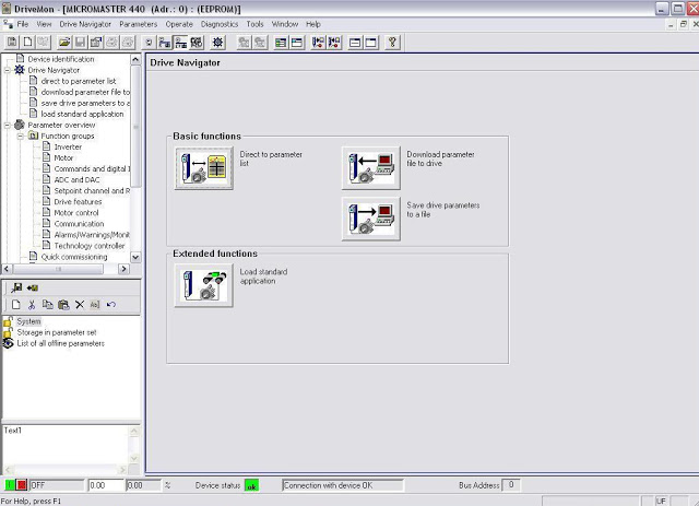
3. Open DriveMon Software & go to FileàSet up an USS ONLINE connection as shown below:

4. In window click on Start (After this software will detect online drive automatically and will go online:

5. Check Device Status.

6. For taking parameter back up click on:

7. Select option “Basic Device complete”:

8. Save parameter file to required location:

9. Wait till upload finishes.:


11. For restoring parameter back up Click on
12. Select the back up parameter file to be restored and click OK.

13. Wait till Download finishes.
Discrete and Continuous speed control using VFDs:
Select the proper size for the load. When specifying VFD size and power ratings, consider the operating profile of the load it will drive. Will the loading be constant or variable? Will there be frequent starts and stops, or will operation be continuous? Consider both torque and peak current. Obtain the highest peak current under the worst operating conditions. Check the motor FLA, which is located on the motor's nameplate. Note that if a motor has been rewound, its FLA may be higher than what's indicated on the nameplate. Don't size the VFD according to horsepower ratings. Instead, size the VFD to the motor at its maximum current requirements at peak torque demand. The VFD must satisfy the maximum demands placed on the motor. Consider the possibility that VFD oversizing may be necessary. Some applications experience temporary overload conditions because of impact loading or starting requirements. Motor performance is based on the amount of current the VFD can produce. For example, a fully-loaded conveyor may require extra breakaway torque, and consequently increased power from the VFD. Many VFDs are designed to operate at 150% overload for 60 seconds. An application that requires an overload greater than 150%, or for longer than 60 seconds, requires an oversized VFD. Altitude also influences VFD sizing, because VFDs are air-cooled. Air thins at high altitudes, which decreases its cooling properties. Most VFDs are designed to operate at 100% capacity up to an altitude of 1,000 meters; beyond that, the drive must be derated or oversized. Be aware of braking requirements.
Duration: - 240 Hours Content of the Training: The training program is broadly divided into six sessions. Each session is taken by experts with industry experience. As the world of automation is intensifying as each day progresses, engineers can't survive without proper training from the ground level to the advanced level. Our course is highly practical-oriented, aimed at supporting and encouraging fresh engineers to foray into the automation industry and fine tune each engineer personnel.
Six major sessions in which training imparted are:
•Electrical drives and controls.
•Field Instrumentation
•Programmable Logic Controllers (PLC) - Allen-Bradley, Siemens, ABB, Telemecanique PLCs
•Supervisory Control and Data Acquisition (SCADA).
•Introduction to Distributed Control System (DCS) •Control panel designing. 1. Electrical drives and controls
•Basics of Relays, Contactor, MCB, MCCB, ELCB, ACB,SDF etc •Working details of different types of Electric Motors.
•Designing of control circuits using Contactors, Relays, Timers etc •DOL, Star Delta Starter designing for 3 phase motors with specification. •Practical wiring session on different controls.
•Motor drives- AC drives and DC drives.
•Programming and installation of VFDs.
•Discrete and Continuous speed control using VFDs.
•Safety and management concepts of designing a project.
2. Field Instrumentation
•Different types of sensors- analog and discrete
•Technical terms used in instrumentation
•Calibration and testing of sensors- thermo couples, RTD, pressure gauge, level sensors, proximity switches, limit switches etc
•Final control elements- Solenoid valve, control valve, motor actuators, Solenoids, bellows, manual valves etc
•Wiring and commissioning of reactor plant with PLC and SCADA control
3. Programmable Logic Controllers (PLC)
•Architecture of PLC- different modules, power supply unit etc •Need of PLC in designing.
•Different types of sensors- sinking, sourcing, NPN, PNP. •Monitoring the process through sensors- connection details.
•Analog addressing continues process monitoring and control.
•Different types of controllers- ON/OFF, Proportional, Derivative, Integral and PID control.
•PLC Programming of branded PLCs.
•NO/ NC concept. •Data file handling- forcing I/O.
•Wiring and fault correction.
•Programming practices.
4. Supervisory Control And Data Acquisition (SCADA).
•SCADA Packages
•Role of SCADA in industrial automation
•SCADA system configuration, RTU, communication protocols.
•Script programming.
•Real time and historical trend.
•Configuring Alarms.
•Real time project development with PLC interfacing.
•Communication with other software.
•Recipe management.
•Accessing different security levels.
•Report generation of current plant.
5 . Introduction to DCS
•Architecture of DCS
•Yokogawa Centum CS 3000
•Comparison of PLC with DCS
•Programming languages for DCS
•Different types of cards and their functions
6 . Control Panel Designing
•Different types of panels.
•Basic components to be installed in a panel.
•Wiring details of panel.
•Specification and physical dimension of components.
•Earthing and Cabling of Panels- standard procedures.
•P&I diagram
1. Electrical drives and controls
= = = = = = = = = = = = = = = = = = = = = = = = = = = = = = = = = = = = = = = = = = = = = = = = = = = = = =
Basics of Relays, Contactor, MCB, MCCB, ELCB, RCD, ACB
Relays:
A relay is an electrically operated switch. Many relays use an electromagnet to operate a switching mechanism mechanically, but other operating principles are also used. Relays are used where it is necessary to control a circuit by a low-power signal (with complete electrical isolation between control and controlled circuits), or where several circuits must be controlled by one signal.

Relay-1, Relay-2
A contactor is an electrically controlled switch used for switching a power circuit, similar to a relay except with higher current ratings.A contactor is controlled by a circuit which has a much lower power level than the switched circuit.

For better Understanding click the following links:
Link-1, Link-2
MCB:
For better Understanding click the following links:
Link-1, Link-2
MCB:
A circuit breaker is an automatically operated electrical switch designed to protect an electrical circuit from damage caused by overload or short circuit. Its basic function is to detect a fault condition and interrupt current flow. Unlike a fuse, which operates once and then must be replaced, a circuit breaker can be reset (either manually or automatically) to resume normal operation. Circuit breakers are made in varying sizes, from small devices that protect an individual household appliance up to large switch-gear designed to protect high-voltage circuits feeding an entire city

For better Understanding click the following links: Link-1, Link-2, Link-3
For better Understanding click the following links: Link-1, Link-2, Link-3
MCCB:
Molded case circuit breakers provide circuit over-current protection with inverse time and instantaneous tripping characteristics. MCCB’s have a quick-make, quick-break over center toggle type mechanism and the handle mechanism shall be trip free to prevent holding contacts closed against a short circuit or sustained overload. MCCB handles assume a position between “ON” and “OFF” when tripped automatically. Multi-pole circuit breakers have common-trip such that an overload or short circuit on any one pole will result in all poles opening simultaneously. Shunt trips, bell alarms, and auxiliary switches are provided. Gold plated auxiliary switches shall be supplied for PLC connection. Internal accessories for all breakers shall be UL listed for field installation and modification.
Molded case circuit breakers provide circuit over-current protection with inverse time and instantaneous tripping characteristics. MCCB’s have a quick-make, quick-break over center toggle type mechanism and the handle mechanism shall be trip free to prevent holding contacts closed against a short circuit or sustained overload. MCCB handles assume a position between “ON” and “OFF” when tripped automatically. Multi-pole circuit breakers have common-trip such that an overload or short circuit on any one pole will result in all poles opening simultaneously. Shunt trips, bell alarms, and auxiliary switches are provided. Gold plated auxiliary switches shall be supplied for PLC connection. Internal accessories for all breakers shall be UL listed for field installation and modification.
Circuit breakers 2000 Ampere and below shall have thermal-magnetic trip units, with inverse time-current characteristics. Automatic operation of these circuit breakers shall be obtained by means of thermal magnetic tripping devices located in each pole providing inverse time delay and instantaneous circuit protection. Circuit breakers shall be ambient compensating in that, as the ambient temperature increases over 40ºC, the circuit breaker automatically de-rates itself so as to better protect its associated conductor.
Thermal-magnetic breakers from 250 to 2000A frames shall have thermal interchangeable trip units, with instantaneous magnetic trip settings that are adjustable and accessible from the front of all circuit breakers on frame sizes 250 Amperes and above. Where indicated, provide circuit breakers UL listed for application at 100% of their continuous ampere rating in their intended enclosure.

For better Understanding click the following links:
ELCB: An earth leakage circuit breaker (ELCB) is a device with two earth terminals used to directly detect currents leaking to earth from an installation and cut the power. They were mainly used on TT earthing systems. By having the assumption of the presence of current in the earth line, it means there is any leaking current from the main incoming live cable, thus the power has to be cut off to ensure the safety. State of ELCB when it cuts the power is called tripped. Every time the ELCB tripped, we can reset it back (Connect back the power line) by resetting the trip button.

RCD:
A residual-current device (RCD), or residual-current circuit breaker (RCCB), is an electrical wiring device that disconnects a circuit whenever it detects that the electric current is not balanced between the energized conductor and the return neutral conductor. Such an imbalance may indicate current leakage through the body of a person who is grounded and accidentally touching the energized part of the circuit. A lethal shock can result from these conditions. RCCBs are designed to disconnect quickly enough to prevent injury caused by such shocks. They are not intended to provide protection against over current (overload) or short-circuit conditions.

For better Understanding click the following links: Link-1
ACB:
For better Understanding click the following links: Link-1
ACB:
This type of circuit breakers, is those kind of circuit breaker which operates in air at atmospheric pressure. After development of oil breaker, the medium voltage air circuit breaker (ACB) is replaced completely by oil circuit breakerin different countries. But in countries like France and Italy, ACBs are still preferable choice up to voltage 15 KV. It is also good choice to avoid the risk of oil fire, in case of oil circuit breaker. In America ACBs were exclusively used for the system up to 15 KV until the development of new vacuum and SF6 circuit breakers.

Working principle of Air Circuit Breaker: The working principle of this breaker is rather different from those in any other types of circuit breakers. The main aim of all kind of circuit breaker is to prevent the reestablishment of arcing after current zero by creating a situation where in the contact gap will withstand the system recovery voltage. The air circuit breaker does the same but in different manner. For interrupting arc it creates an arc voltage in excess of the supply voltage. Arc voltage is defined as the minimum voltage required maintaining the arc. This circuit breaker increases the arc voltage by mainly three different ways,It may increase the arc voltage by cooling the arc plasma. As the temperature of arc plasma is decreased, the mobility of the particle in arc plasma is reduced; hence more voltage gradient is required to maintain the arc. It may increase the arc voltage by lengthening the arc path. As the length of arc path is increased, the resistance of the path is increased, and hence to maintain the same arc current more voltage is required to be applied across the arc path. That means arc voltage is increased. Splitting up the arc into a number of series arcs also increases the arc voltage. Types of ACB: There are mainly two types of ACB are available. 1) Plain air circuit breaker 2) Air blast Circuit Breaker. Operation of ACB: The first objective is usually achieved by forcing the arc into contact with as large an area as possible of insulating material. Every air circuit breaker is fitted with a chamber surrounding the contact. This chamber is called ‘arc chute’. The arc is driven into it. If inside of the arc chute is suitably shaped, and if the arc can be made conform to the shape, the arc chute wall will help to achieve cooling. This type of arc chute should be made from some kind of refractory material. High temperature plastics reinforced with glass fiber and ceramics are preferable materials for making arc chute. The second objective that is lengthening the arc path, is achieved concurrently with fist objective. If the inner walls of the arc chute is shaped in such a way that the arc is not only forced into close proximity with it but also driven into a serpentine channel projected on the arc chute wall. The lengthening of the arc path increases the arc resistance. The third technique is achieved by using metal arc slitter inside the arc chute. The main arc chute is divided into numbers of small compartments by using metallic separation plates. These metallic separation plates are actually the arc splitters and each of the small compartments behaves as individual mini arc chute. In this system the initial arc is split into a number of series arcs, each of which will have its won mini arc chute. So each of the split arcs has its won cooling and lengthening effect due to its won mini arc chute and hence individual split arc voltage becomes high. These collectively, make the over all arc voltage, much higher than the system voltage. This was working principle of air circuit breaker now we will discuss in details the operation of ACB in practice. The air circuit breaker, operated within the voltage level 1KV, does not require any arc control device. Mainly for heavy fault current on low voltages (low voltage level above 1 KV) ABCs with appropriate arc control device, are good choice. These breakers normally have two pairs of contacts. The main pair of contacts carries the current at normal load and these contacts are made of copper. The additional pair is the arcing contact and is made of carbon. When circuit breaker is being opened, the main contacts open first and during opening of main contacts the arcing contacts are still in touch with each other. As the current gets, a parallel low resistive path through the arcing contact during opening of main contacts, there will not be any arcing in the main contact. The arcing is only initiated when finally the arcing contacts are separated. The each of the arc contacts is fitted with an arc runner which helps, the arc discharge to move upward due to both thermal and electromagnetic effects as shown in the figure. As the arc is driven upward it enters in the arc chute, consisting of splitters. The arc in chute will become colder, lengthen and split hence arc voltage becomes much larger than system voltage at the time of operation of air circuit breaker, and therefore the arc is quenched finally during the current zero. Although this type of circuit breakers have become obsolete for medium voltage application, but they are still preferable choice for high current rating in low voltage application.
Working principle of Air Circuit Breaker: The working principle of this breaker is rather different from those in any other types of circuit breakers. The main aim of all kind of circuit breaker is to prevent the reestablishment of arcing after current zero by creating a situation where in the contact gap will withstand the system recovery voltage. The air circuit breaker does the same but in different manner. For interrupting arc it creates an arc voltage in excess of the supply voltage. Arc voltage is defined as the minimum voltage required maintaining the arc. This circuit breaker increases the arc voltage by mainly three different ways,It may increase the arc voltage by cooling the arc plasma. As the temperature of arc plasma is decreased, the mobility of the particle in arc plasma is reduced; hence more voltage gradient is required to maintain the arc. It may increase the arc voltage by lengthening the arc path. As the length of arc path is increased, the resistance of the path is increased, and hence to maintain the same arc current more voltage is required to be applied across the arc path. That means arc voltage is increased. Splitting up the arc into a number of series arcs also increases the arc voltage. Types of ACB: There are mainly two types of ACB are available. 1) Plain air circuit breaker 2) Air blast Circuit Breaker. Operation of ACB: The first objective is usually achieved by forcing the arc into contact with as large an area as possible of insulating material. Every air circuit breaker is fitted with a chamber surrounding the contact. This chamber is called ‘arc chute’. The arc is driven into it. If inside of the arc chute is suitably shaped, and if the arc can be made conform to the shape, the arc chute wall will help to achieve cooling. This type of arc chute should be made from some kind of refractory material. High temperature plastics reinforced with glass fiber and ceramics are preferable materials for making arc chute. The second objective that is lengthening the arc path, is achieved concurrently with fist objective. If the inner walls of the arc chute is shaped in such a way that the arc is not only forced into close proximity with it but also driven into a serpentine channel projected on the arc chute wall. The lengthening of the arc path increases the arc resistance. The third technique is achieved by using metal arc slitter inside the arc chute. The main arc chute is divided into numbers of small compartments by using metallic separation plates. These metallic separation plates are actually the arc splitters and each of the small compartments behaves as individual mini arc chute. In this system the initial arc is split into a number of series arcs, each of which will have its won mini arc chute. So each of the split arcs has its won cooling and lengthening effect due to its won mini arc chute and hence individual split arc voltage becomes high. These collectively, make the over all arc voltage, much higher than the system voltage. This was working principle of air circuit breaker now we will discuss in details the operation of ACB in practice. The air circuit breaker, operated within the voltage level 1KV, does not require any arc control device. Mainly for heavy fault current on low voltages (low voltage level above 1 KV) ABCs with appropriate arc control device, are good choice. These breakers normally have two pairs of contacts. The main pair of contacts carries the current at normal load and these contacts are made of copper. The additional pair is the arcing contact and is made of carbon. When circuit breaker is being opened, the main contacts open first and during opening of main contacts the arcing contacts are still in touch with each other. As the current gets, a parallel low resistive path through the arcing contact during opening of main contacts, there will not be any arcing in the main contact. The arcing is only initiated when finally the arcing contacts are separated. The each of the arc contacts is fitted with an arc runner which helps, the arc discharge to move upward due to both thermal and electromagnetic effects as shown in the figure. As the arc is driven upward it enters in the arc chute, consisting of splitters. The arc in chute will become colder, lengthen and split hence arc voltage becomes much larger than system voltage at the time of operation of air circuit breaker, and therefore the arc is quenched finally during the current zero. Although this type of circuit breakers have become obsolete for medium voltage application, but they are still preferable choice for high current rating in low voltage application.
Air Blast Circuit Breaker These types of air circuit breaker were used for the system voltage of 245KV, 420KV and even more, especially where faster breaker operation was required. Air Blast Circuit Breaker has some specific advantages over oil circuit breaker which are listed as follows,
1) There is no chance of fire hazard caused by oil.
2) The breaking speed of circuit breaker is much higher during operation of air blast circuit breaker.
3) Arc quenching is much faster during operation of air blast circuit breaker.
4) The duration of arc is same for all values of small as well as high currents interruptions.
5) As the duration of arc is smaller, so lesser amount of heat realized from arc to current carrying contacts hence the service life of the contacts becomes longer.
6) The stability of the system can be well maintained as it depends on the speed of operation of circuit breaker.
7) Requires much less maintenance compared to oil circuit breaker.
There are also some disadvantages of air blast circuit breakers
1) In order to have frequent operations, it is necessary to have sufficiently high capacity air compressor.
2) Frequent maintenance of compressor, associated air pipes and automatic control equipments is also required.
3) Due to high speed current interruption there is always a chance of high rate of rise of re-striking voltage and current chopping.
4) There also a chance of air pressure leakage from air pipes junctions. As we said earlier that there are mainly two types of ACB, plain air circuit breaker and air blast circuit breaker. But the later can be sub divided further into three different categories. a)Axial Blast ACB. b) Axial Blast ACB with side moving contact. c) Cross Blast ACB.
Axial Blast Air Circuit Breaker :

In Axial Blast ACB the moving contact is in contact with fixed contact with the help of a spring pressure as shown in the figure. There is a nozzle orifice in the fixed contact which is blocked by tip of the moving contact at normal closed condition of the breaker. When fault occurs, the high pressure air is introduced into the arcing chamber. The air pressure will counter the spring pressure and deforms the spring hence the moving contact is withdrawn from the fixed contact and nozzle hole becomes open. At the same time the high pressure air starts flowing along the arc through the fixed contact nozzle orifice. This axial flow of air along the arc through the nozzle orifice will make the arc lengthen and colder hence arc voltage become much higher than system voltage that means system voltage is insufficient to sustain the arc consequently the arc is quenched.

Axial Blast ACB with side moving contact In this type of axial blast air circuit breaker the moving contact is fitted over a piston supported over a spring. In order to open the circuit breaker the air is admitted into the arcing chamber when pressure reaches to a predetermined value, it presses down the moving contact; an arc is drawn between the fixed and moving contacts. The air blast immediately transfers the arc to the arcing electrode and is consequently quenched by the axial flow of air.
Cross Blast Air Circuit Breaker:

The working principle of Cross Blast Air Circuit Breaker is quite simple. In this system of air blast circuit breaker the blast pipe is fixed in perpendicular to the movement of moving contact in the arcing chamber and on the opposite side of the arcing chamber one exhaust chamber is also fitted at the same alignment of blast pipe, so that the air comes from blast pipe can straightly enter into exhaust chamber through the contact gap of the breaker. The exhaust chamber is spit with arc splitters. When moving contact is withdrawn from fixed contact, an arc is established in between the contact, and at the same time high pressure air coming from blast pipe will pass through the contact gap and will forcefully take the arc into exhaust chamber where the arc is split with the help of arc splitters and ultimately arc is quenched.
For better Understanding click the following links: Link-1
2) The breaking speed of circuit breaker is much higher during operation of air blast circuit breaker.
3) Arc quenching is much faster during operation of air blast circuit breaker.
4) The duration of arc is same for all values of small as well as high currents interruptions.
5) As the duration of arc is smaller, so lesser amount of heat realized from arc to current carrying contacts hence the service life of the contacts becomes longer.
6) The stability of the system can be well maintained as it depends on the speed of operation of circuit breaker.
7) Requires much less maintenance compared to oil circuit breaker.
There are also some disadvantages of air blast circuit breakers
1) In order to have frequent operations, it is necessary to have sufficiently high capacity air compressor.
2) Frequent maintenance of compressor, associated air pipes and automatic control equipments is also required.
3) Due to high speed current interruption there is always a chance of high rate of rise of re-striking voltage and current chopping.
4) There also a chance of air pressure leakage from air pipes junctions. As we said earlier that there are mainly two types of ACB, plain air circuit breaker and air blast circuit breaker. But the later can be sub divided further into three different categories. a)Axial Blast ACB. b) Axial Blast ACB with side moving contact. c) Cross Blast ACB.
Axial Blast Air Circuit Breaker :
In Axial Blast ACB the moving contact is in contact with fixed contact with the help of a spring pressure as shown in the figure. There is a nozzle orifice in the fixed contact which is blocked by tip of the moving contact at normal closed condition of the breaker. When fault occurs, the high pressure air is introduced into the arcing chamber. The air pressure will counter the spring pressure and deforms the spring hence the moving contact is withdrawn from the fixed contact and nozzle hole becomes open. At the same time the high pressure air starts flowing along the arc through the fixed contact nozzle orifice. This axial flow of air along the arc through the nozzle orifice will make the arc lengthen and colder hence arc voltage become much higher than system voltage that means system voltage is insufficient to sustain the arc consequently the arc is quenched.
Axial Blast ACB with side moving contact In this type of axial blast air circuit breaker the moving contact is fitted over a piston supported over a spring. In order to open the circuit breaker the air is admitted into the arcing chamber when pressure reaches to a predetermined value, it presses down the moving contact; an arc is drawn between the fixed and moving contacts. The air blast immediately transfers the arc to the arcing electrode and is consequently quenched by the axial flow of air.
Cross Blast Air Circuit Breaker:
The working principle of Cross Blast Air Circuit Breaker is quite simple. In this system of air blast circuit breaker the blast pipe is fixed in perpendicular to the movement of moving contact in the arcing chamber and on the opposite side of the arcing chamber one exhaust chamber is also fitted at the same alignment of blast pipe, so that the air comes from blast pipe can straightly enter into exhaust chamber through the contact gap of the breaker. The exhaust chamber is spit with arc splitters. When moving contact is withdrawn from fixed contact, an arc is established in between the contact, and at the same time high pressure air coming from blast pipe will pass through the contact gap and will forcefully take the arc into exhaust chamber where the arc is split with the help of arc splitters and ultimately arc is quenched.
For better Understanding click the following links: Link-1
The motor or an electrical motor is a device that has brought about one of the biggest advancements in the fields of engineering and technology ever since the invention of electricity. A motor is nothing but an electro-mechanical device that converts electrical energy to mechanical energy. Its because of motors, life is what it is today in the 21st century. Without motor we had still been living in Sir Thomas Edison’s Era where the only purpose of electricity would have been to glow bulbs. There are different types of motor have been developed for different specific purposes. In simple words we can say a device that produces rotational force is a motor. The very basic principal of functioning of an electrical motor lies on the fact that force is experienced in the direction perpendicular to magnetic field and the current, when field and electric current are made to interact with each other. Ever since the invention of motors, a lot of advancements has taken place in this field of engineering and it has become a subject of extreme importance for modern engineers. This particular webpage takes into consideration, the above mentioned fact and provides a detailed description on all major electrical motors and motoring parts being used in the present era. Motor Starting and Running Currents and Rating Guide: A word of caution: The following article is based on National Electrical Manufacturers' Association (NEMA) tables, standards and nomenclature. This is somewhat different from Indian and European practice. The class designations are applicable only to NEMA compatible motors which are in use in the US only. However, the logic and pattern of calculations are the same everywhere. Hence the reader is cautioned to follow only the logical sequence of the calculations. Motor Starting Current: When typical induction motors become energized, a much larger amount of current than normal operating current rushes into the motor to set up the magnetic field surrounding the motor and to overcome the lack of angular momentum of the motor and its load. As the motor increases to slip speed, the current drawn subsides to match (1) the current required at the supplied voltage to supply the load and (2) losses to windage and friction in the motor and in the load and transmission system. A motor operating at slip speed and supplying nameplate horsepower as the load should draw the current printed on the nameplate, and that current should satisfy the equation
Horsepower = (voltage X current X power factor X motor efficiency X v3) / 746
Typical induction motors exhibit a starting power factor of 10 to 20 percent and a full-load running power factor of 80 to 90 percent. Smaller typical induction motors exhibit an operating full-load efficiency of approximately 92 percent, whereas large typical induction motors exhibit an operating full-load efficiency of approximately 97.5 percent.
Typical induction motors exhibit a starting power factor of 10 to 20 percent and a full-load running power factor of 80 to 90 percent. Smaller typical induction motors exhibit an operating full-load efficiency of approximately 92 percent, whereas large typical induction motors exhibit an operating full-load efficiency of approximately 97.5 percent.
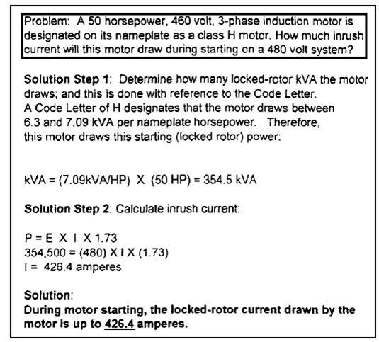
Since many types of induction motors are made, the inrush current from an individual motor is important in designing the electrical power supply system for that motor. For this purpose, the nameplate on every motor contains a code letter indicating the kilovoltampere/horsepower starting load rating of the motor. A table of these code letters and their meanings in approximate kVA and horsepower is shown in the following table.
Using these values, the inrush current for a specific motor can be calculated as
Because of the items listed above, motors that produce constant kVA loads make demands on the electrical power system that are extraordinary compared with the demands of constant kilowatt loads. To start them, the over current protection system must permit the starting current, also called the locked-rotor current, to flow during the normal starting period, and then the motor-running over current must be limited to approximately the nameplate full-load ampere rating. If the duration of the locked-rotor current is too long, the motor will overheat due to I2R heat buildup, and if the long-time ampere draw of the motor is too high, the motor also will overheat due to I2R heating. The National Electrical Code provides limitations on both inrush current and running current, as well as providing a methodology to determine motor disconnect switch ampere and horsepower ratings.
Motor Running Current:
Calculating Motor Branch-Circuit Overcurrent Protection and Wire Size
A 40 HP, 460 V, 3 phase, Code letter G, Service factor of 1.0 is planned for operation from a 460 V, 3 phase system. The name plate ampere is 50A. The motor is rated for continuous duty and the load is continuous. Solve for minimum sizes of branch circuit elements?
NEC Torque classes and characteristics
Classification or Types of Motor The primary classification of motor or types of motor can be tabulated as shown below,
 History of Motor In the year 1821 British scientist Michael Faraday explained the conversion of electrical energy into mechanical energy by placing a current carrying conductor in a magnetic field which resulted in the rotation of the conductor due to torque produced by the mutual action of electrical current and field. Based on his principal the most primitive of machines a D.C.(direct current) machine was designed by another British scientist William Sturgeon in the year 1832. But his model was overly expensive and wasn’t used for any practical purpose. Later in the year 1886 the first electrical motor was invented by scientist Frank Julian Sprague. That was capable of rotating at a constant speed under a varied range of load, and thus derived motoring action.
INDEX
1) DC Motor
2) Synchronous Motor
3) 3 Phase Induction Motor
4) 1 Phase Induction Motor
5) Special Types of Motor Among the four basic classification of motors mentioned above the DC motor as the name suggests, is the only one that is driven by direct current. It’s the most primitive version of the electric motor where rotating torque is produced due to flow of electric current through the conductor inside a magnetic field. Rest all are A.C. electrical motors, and are driven by alternating current, for e.g. the synchronous motor, which always runs at synchronous speed. Here the rotor is an Electromagnet which is magnetically locked with stator rotating magnetic field and rotates with it. The speed of these machines are varied by varying the frequency (f) and number of poles (P), as Ns = 120 f/P. In another type of AC motor where rotating magnetic field cuts the rotor conductors, hence circulating current induced in these short circuited rotor conductors. Due to interaction of the magnetic field and these circulating currents the rotor starts rotates and continues its rotation. This is induction motor which is also known as asynchronous motor runs at a speed lesser than synchronous speed, and the rotating torque, and speed is governed by varying the slip which gives the difference between synchronous speed Ns , and rotor speed speed Nr, It runs governing the principal of EMF induction due to varying flux density, hence the name induction machine comes. Single phase induction motor like a 3 phase, runs by the principal of emf induction due to flux, but the only difference is, it runs on single phase supply and its starting methods are governed by two well established theories, namely the Double Revolving field theory and the Cross field theory. Apart from the four basic types of motor mentioned above, there are several types Of special electrical motors like Linear Induction motor(LIM),Stepper motor, Servo motor etc with special features that has been developed according to the needs of the industry or for a particular particular gadget like the use of hysteresis motor in hand watches because of its compactness.
Code Letter on motor name plate
|
kVA per HP with locked rotor
|
||
Minimum
|
Mean
|
Maximum
|
|
A
|
0
|
1.57
|
3.14
|
B
|
3.15
|
3.345
|
3.54
|
C
|
3.55
|
3.77
|
3.99
|
D
|
4
|
4.245
|
4.9
|
E
|
4.5
|
4.745
|
4.99
|
F
|
5
|
5.295
|
5.59
|
G
|
5.6
|
5.945
|
6.29
|
H
|
6.3
|
6.695
|
7.09
|
J
|
7.1
|
7.545
|
7.99
|
K
|
8
|
8.495
|
8.9
|
L
|
9
|
9.495
|
9.9
|
M
|
10
|
10.595
|
11.19
|
N
|
11.2
|
11.845
|
12.49
|
P
|
12.5
|
13.245
|
13.99
|
R
|
14
|
14.995
|
15.99
|
S
|
16
|
16.995
|
17.99
|
T
|
18
|
18.995
|
19.99
|
U
|
20
|
29.2
|
22.39
|
V
|
22.4
|
No Limit
|
No Limit
|
Using these values, the inrush current for a specific motor can be calculated as
Iinrush=(code letter value X horse power x 1000) /( v3 X Voltage)
An example of this calculation for a 50-hp code letter G motor operating at 460 V is shown below

Because of the items listed above, motors that produce constant kVA loads make demands on the electrical power system that are extraordinary compared with the demands of constant kilowatt loads. To start them, the over current protection system must permit the starting current, also called the locked-rotor current, to flow during the normal starting period, and then the motor-running over current must be limited to approximately the nameplate full-load ampere rating. If the duration of the locked-rotor current is too long, the motor will overheat due to I2R heat buildup, and if the long-time ampere draw of the motor is too high, the motor also will overheat due to I2R heating. The National Electrical Code provides limitations on both inrush current and running current, as well as providing a methodology to determine motor disconnect switch ampere and horsepower ratings.
Table 430-152 of the National Electrical Code provides the maximum setting of over current devices upstream of the motor branch circuit, and portions of this table are replicated below:
% of Full load current
|
||||
Motor type
|
Single element fuse
|
Dual-element time delay fuse
|
Inverse time breaker
|
Instantaneous & Magnetic trip breaker
|
Single phase motor
|
300
|
175
|
250
|
800
|
Three phase squirrel cage motor
|
300
|
175
|
250
|
800
|
Design E three phase squirrel cage
|
300
|
175
|
250
|
1100
|
Synchronous
|
300
|
175
|
250
|
800
|
Wound rotor
|
150
|
150
|
150
|
800
|
Direct current
|
150
|
150
|
150
|
250
|
For example, a 50 hp, Design B, 460V 3 phase motor has a full load current of 65A at 460V. The maximum rating of an inverse time breaker protecting the motor branch circuit would be 65A x 250%, or 162.5A. The next higher standard rating is 175A (US), so 175A is the maximum rating that can be used to protect the motor circuit.
|
||||
Motor Running Current:
The following figures illustrate the calculations required by specific types of motors in the design of electric circuits to permit these loads to start and to continue to protect them during operation.
Table of full-load currents for three-phase ac induction motors (A part of table 430-150 of NEC).
HP
|
208 V
|
230 V
|
460 V
|
575 V
|
0.5
|
2.5
|
2.2
|
1.1
|
0.9
|
0.75
|
3.5
|
3.2
|
1.6
|
1.3
|
1
|
4.6
|
4.2
|
2.1
|
1.7
|
1.5
|
6.6
|
6
|
3
|
2.4
|
2
|
7.5
|
6.8
|
3.4
|
2.7
|
3
|
10.6
|
9.6
|
4.8
|
3.9
|
5
|
16.7
|
15.2
|
7.6
|
6.1
|
10
|
30.8
|
28
|
14
|
11
|
15
|
46.2
|
42
|
21
|
17
|
20
|
59.4
|
54
|
27
|
22
|
25
|
74.8
|
68
|
34
|
27
|
30
|
88
|
80
|
40
|
32
|
40
|
114
|
104
|
52
|
41
|
50
|
143
|
130
|
65
|
52
|
60
|
169
|
154
|
77
|
62
|
75
|
211
|
192
|
96
|
77
|
100
|
273
|
248
|
124
|
99
|
125
|
343
|
312
|
156
|
125
|
150
|
396
|
360
|
180
|
144
|
200
|
528
|
480
|
240
|
192
|
Calculating Motor Branch-Circuit Overcurrent Protection and Wire Size
Article 430-52 of the National Electrical Code specifies that the minimum motor branch-circuit size must be rated at 125 percent of the motor full-load current found in Table 430-150 for motors that operate continuously, and Section 430-32 requires that the long-time overload trip rating not be greater than 115 percent of the motor nameplate current unless the motor is marked otherwise. Note that the values of branch-circuit over current trip (the long-time portion of a thermal-magnetic trip circuit breaker and the fuse melt-out curve ampacity) are changed by Table 430-22b for motors that do not operate continuously.
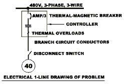
This is illustrated with a sample problem. Consider the circuit shown.

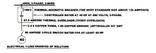
A 40 HP, 460 V, 3 phase, Code letter G, Service factor of 1.0 is planned for operation from a 460 V, 3 phase system. The name plate ampere is 50A. The motor is rated for continuous duty and the load is continuous. Solve for minimum sizes of branch circuit elements?
1. Take motor full load current from table 430-150 as 52A which is higher than name plate value.
2. Determine wire size: 125% of 52A = 65A.
3. Determine inverse time breaker setting: 250% of 52A = 130A, next standard rating is 150A.
4. Determine the rating of thermal overloads: 115% of 50A (name plate current) = 57.5 A
5. Determine disconnect switch ampere rating: 115% of 52A = 59.8 A
6. Determine controller HP rating: 40 HP (same as motor nameplate HP)
The completed circuit will look like this.

NEC Torque classes and characteristics
Design Letter
|
Starting current (%FLC)
|
Relative Efficiency
|
Slip in % rpm
|
Starting torque (%FLT)
|
Stalling torque (%FLT)
|
A
|
Depends upon-name plate-code letter Normally 630-1000%
|
High
|
3%
|
120-250%
|
200-275%
|
B
|
Normally 600-700%
|
High
|
1.5-3%
|
120-250%
|
200-275%
|
C
|
Normally 600-700%
|
High
|
1.5-3%
|
200-250%
|
190-225%
|
D
|
Normally 600-700%
|
Medium
|
5-8%
|
275%
|
275%
|
Classification or Types of Motor The primary classification of motor or types of motor can be tabulated as shown below,

INDEX
1) DC Motor
2) Synchronous Motor
3) 3 Phase Induction Motor
4) 1 Phase Induction Motor
5) Special Types of Motor Among the four basic classification of motors mentioned above the DC motor as the name suggests, is the only one that is driven by direct current. It’s the most primitive version of the electric motor where rotating torque is produced due to flow of electric current through the conductor inside a magnetic field. Rest all are A.C. electrical motors, and are driven by alternating current, for e.g. the synchronous motor, which always runs at synchronous speed. Here the rotor is an Electromagnet which is magnetically locked with stator rotating magnetic field and rotates with it. The speed of these machines are varied by varying the frequency (f) and number of poles (P), as Ns = 120 f/P. In another type of AC motor where rotating magnetic field cuts the rotor conductors, hence circulating current induced in these short circuited rotor conductors. Due to interaction of the magnetic field and these circulating currents the rotor starts rotates and continues its rotation. This is induction motor which is also known as asynchronous motor runs at a speed lesser than synchronous speed, and the rotating torque, and speed is governed by varying the slip which gives the difference between synchronous speed Ns , and rotor speed speed Nr, It runs governing the principal of EMF induction due to varying flux density, hence the name induction machine comes. Single phase induction motor like a 3 phase, runs by the principal of emf induction due to flux, but the only difference is, it runs on single phase supply and its starting methods are governed by two well established theories, namely the Double Revolving field theory and the Cross field theory. Apart from the four basic types of motor mentioned above, there are several types Of special electrical motors like Linear Induction motor(LIM),Stepper motor, Servo motor etc with special features that has been developed according to the needs of the industry or for a particular particular gadget like the use of hysteresis motor in hand watches because of its compactness.

Electrical Motor,
Working of ElectricMotor,
DC Motor,
Working Principle of DCMotor
Construction of DCMotor
Torque Equation of DC Motor
Types of DC Motor
Shunt Wound DC Motor
Series Wound DC Motor
Compound Wound DC Motor
Starting Methods of DCMotor
Three Point Starter
Four Point Starter
Speed Regulation of DC Motor
Speed Control of DCMotor
Three Phase InductionMotor
Linear Induction Motor
Synchronous Motor
Synchronous MotorExcitation
Hunting in SynchronousMotor
Motor Generator Set
Designing of control circuits using Contactors, Relays, Timers etc:

Using Relay:


DOL, Star Delta Starter designing for 3 phase motors with specification:
DOL Starter:

Different starting methods are employed for starting induction motors because Induction Motor draws more starting current during starting. To prevent damage to the windings due to the high starting current flow, we employ different types of starters.
The simplest form of motor starter for the induction motor is the Direct On Line starter. The Direct On Line Motor Starter (DOL) consist a MCCB or Circuit Breaker, Contactor and an overload relay for protection. Electromagnetic contactor which can be opened by the thermal overloa relay under fault conditions.
Typically, the contactor will be controlled by separate start and stop buttons, and an auxiliary contact on the contactor is used, across the start button, as a hold in contact. I.e. the contactor is electrically latche closed while the motor is operating. Principle of Direct On Line Starter (DOL):
To start, the contactor is closed, applying full line voltage to the motor windings. The motor will draw a very high inrush current for a very short time, the magnetic field in the iron, and then the current will be limited to the Locked Rotor Current of the motor. The motor will develop Locked Rotor Torque and begin to accelerate towards full speed.
As the motor accelerates, the current will begin to drop, but will not drop significantly until the motor is at a high speed, typically about 85% of synchronous speed. The actual starting current curve is a function of the motor design, and the terminal voltage, and is totally independent of the motor load.
The motor load will affect the time taken for the motor to accelerate to full speed and therefore the duration of the high starting current, but not the magnitude of the starting current.
Provided the torque developed by the motor exceeds the load torque at all speeds during the start cycle, the motor will reach full speed. If the torque delivered by the motor is less than the torque of the load at any speed during the start cycle, the motor will stops accelerating. If the starting torque with a DOL starter is insufficient for the load, the motor must be replaced with a motor which can develop a higher starting torque.
The acceleration torque is the torque developed by the motor minus the load torque, and will change as the motor accelerates due to the motor speed torque curve and the load speed torque curve. The start time is dependent on the acceleration torque and the load inertia.
Note: DOL starting have a maximum start current and maximum start torque. This may cause an electrical problem with the supply, or it may cause a mechanical problem with the driven load. So this will be inconvenient for the users of the supply line, always experience a voltage drop when starting a motor. But if this motor is not a high power one it does not affect much.
Parts of DOL Starters:
Contactors & Coil:

DOL part -Contactor:
Magnetic contactors are electromagnetically operated switches that provide a safe and convenient means for connecting and interrupting branch circuits.
Magnetic motor controllers use electromagnetic energy for closing switches. The electromagnet consists of a coil of wire placed on an iron core. When a current flow through the coil, the iron of the magnet becomes magnetized, attracting an iron bar called the armature. An interruption of the current flow through the coil of wire causes the armature to drop out due to the presence of an air gap in the magnetic circuit.
Line-voltage magnetic motor starters are electro-mechanical devices that provide a safe, convenient, and economical means of starting and stopping motors, and have the advantage of being controlled remotely. The great bulk of motor controllers sold are of this type.
Contactors are mainly used to control machinery which uses electric motors. It consists of a coil which connects to a voltage source. Very often for Single phase Motors, 230V coils are used and for three phase motors, 415V coils are used. The contactor has three main NO contacts and lesser power rated contacts named as Auxiliary Contacts [NO and NC] used for the control circuit. A contact is conducting metal parts which completes or interrupt an electrical circuit.
NO-normally open
NC-normally closed
Over Load Relay (Overload protection)
Overload protection for an electric motor is necessary to prevent burnout and to ensure maximum operating life.
Under any condition of overload, a motor draws excessive current that causes overheating. Since motor winding insulation deteriorates due to overheating, there are established limits on motor operating temperatures to protect a motor from overheating. Overload relays are employed on a motor control to limit the amount of current drawn.
The overload relay does not provide short circuit protection. This is the function of over current protective equipment like fuses and circuit breakers, generally located in the disconnecting switch enclosure.
The ideal and easiest way for overload protection for a motor is an element with current-sensing properties very similar to the heating curve of the motor which would act to open the motor circuit when full-load current is exceeded. The operation of the protective device should be such that the motor is allowed to carry harmless over-loads but is quickly removed from the line when an overload has persisted too long.
DOL part - Termal Overload Relay:
Normally fuses are not designed to provide overload protection. Fuse is protecting against short circuits (over current protection). Motors draw a high inrush current when starting and conventional fuses have no way of distinguishing between this temporary and harmless inrush current and a damaging overload. Selection of Fuse is depend on motor full-load current, would “blow” every time the motor is started. On the other hand, if a fuse were chosen large enough to pass the starting or inrush current, it would not protect the motor against small, harmful overloads that might occur later.
The overload relay is the heart of motor protection. It has inverse-trip-time characteristics, permitting it to hold in during the accelerating period (when inrush current is drawn), yet providing protection on small overloads above the full-load current when the motor is running. Overload relays are renewable and can withstand repeated trip and reset cycles without need of replacement. Overload relays cannot, however, take the place of over current protection equipment.
The overload relay consists of a current-sensing unit connected in the line to the motor, plus a mechanism, actuated by the sensing unit, which serves, directly or indirectly, to break the circuit.
Overload relays can be classified as being thermal, magnetic, or electronic
Thermal Relay: As the name implies, thermal overload relays rely on the rising temperatures caused by the overload current to trip the overload mechanism. Thermal overload relays can be further subdivided into two types: melting alloy and bimetallic.
Magnetic Relay: Magnetic overload relays react only to current excesses and are not affected by temperature.
Electronic Relay: Electronic or solid-state overload relays, provide the combination of high-speed trip, adjustability, and ease of installation. They can be ideal in many precise applications.
Wiring of DOL Starter:

1. Main Contact
Contactor is connecting among Supply Voltage, Relay Coil and Thermal Overload Relay.
L1 of Contactor Connect (NO) to R Phase through MCCB
L2 of Contactor Connect (NO) to Y Phase through MCCB
L3 of Contactor Connect (NO) to B Phase through MCCB.
NO Contact (-||-):
(13-14 or 53-54) is a normally Open NO contact (closes when the relay energizes)
Contactor Point 53 is connecting to Start Button Point (94) and 54 Point of Contactor is connected to Common wire of Start/Stop Button.
NC Contact (-|/|-): (95-96) is a normally closed NC contact (opens when the thermal overloads trip if associated with the overload block)
2. Relay Coil Connection
A1 of Relay Coil is connecting to any one Supply Phase and
A2 is connecting to Thermal over Load Relay’s NC Connection (95).
3. Thermal Overload Relay Connection:
T1,T2,T3 are connect to Thermal Overload Relay
Overload Relay is Connecting between Main Contactor and Motor
NC Connection (95-96) of Thermal Overload Relay is connecting to Stop Button and Common Connection of Start/Stop Button.
Wiring Diagram of DOL Starter:

Direct On Line Starter - Wiring Diagram
Working principle of DOL Starter
The main heart of DOL starter is Relay Coil. Normally it gets one phase constant from incoming supply Voltage (A1).when Coil get second Phase relay coil energizes and Magnet of Contactor produce electromagnetic field and due to this Plunger of Contactor will move and Main Contactor of starter will closed and Auxiliary will change its position NO become NC and NC become (shown Red Line in Diagram) .
Pushing Start Button:
When We Push the start Button Relay Coil will get second phase from Supply Phase-Main contactor(5)-Auxiliary Contact(53)-Start button-Stop button-96-95-To Relay Coil (A2).Now Coil energizes and Magnetic field produce by Magnet and Plunger of Contactor move. Main Contactor closes and Motor gets supply at the same time Auxiliary contact become (53-54) from NO to NC .
Release Start Button:
Relay coil gets supply even though we release Start button. When We release Start Push Button Relay Coil gets Supply phase from Main contactor (5)-Auxiliary contactor (53) – Auxiliary contactor (54)-Stop Button-96-95-Relay coil (shown Red / Blue Lines in Diagram).
In Overload Condition of Motor will be stopped by intermission of Control circuit at Point 96-95.
Pushing Stop Button:
When we push Stop Button Control circuit of Starter will be break at stop button and Supply of Relay coil is broken, Plunger moves and close contact of Main Contactor becomes Open, Supply of Motor is disconnected.

DOL - Wiring scheme
Motor Starting Characteristics on DOL Starter
Available starting current: 100%.
Peak starting current: 6 to 8 Full Load Current.
Peak starting torque: 100%
Advantages of DOL Starter:
Most Economical and Cheapest Starter
Simple to establish operate and maintain
Simple Control Circuitry
Easy to understand and trouble-shoot.
It provides 100% torque at the time of starting.
Only one set of cable is required from starter to motor.
Motor is connected in delta at motor terminals.
Disadvantages of DOL Starter:
It does not reduce the starting current of the motor.
High Starting Current: Very High Starting Current (Typically 6 to 8 times the FLC of the motor).
Mechanically Harsh: Thermal Stress on the motor, thereby reducing its life.
Voltage Dip: There is a big voltage dip in the electrical installation because of high in-rush current affecting other customers connected to the same lines and therefore not suitable for higher size squirrel cage motors
High starting Torque: Unnecessary high starting torque, even when not required by the load, thereby increased mechanical stress on the mechanical systems such as rotor shaft, bearings, gearbox, coupling, chain drive, connected equipments, etc. leading to premature failure and plant downtimes.
Features of DOL starting:
For low- and medium-power three-phase motors
Three connection lines (circuit layout: star or delta)
High starting torque
Very high mechanical load
High current peaks
Voltage dips
Simple switching devices
Direct On Line Motor Starter (DOL) is suitable for:
A direct on line starter can be used if the high inrush current of the motor does not cause excessive voltage drop in the supply circuit. The maximum size of a motor allowed on a direct on line starter may be limited by the supply utility for this reason. For example, a utility may require rural customers to use reduced-voltage starters for motors larger than 10 kW.
DOL starting is sometimes used to start small water pumps, compressors, fans and conveyor belts.
Direct On Line Motor Starter (DOL) is NOT suitable for:
The peak starting current would result in a serious voltage drop on the supply system
The equipment being driven cannot tolerate the effects of very high peak torque loading
The safety or comfort of those using the equipment may be compromised by sudden starting as, for example, with escalators and lifts.
Star Delta Starter:
Star Delta Starter:

STAR DELTA connection Diagram and Working principle:
Descriptions: A Dual starter connects the motor terminals directly to the power supply. Hence, the motor is subjected to the full voltage of the power supply. Consequently, high starting current flows through the motor. This type of starting is suitable for small motors below 5 hp (3.75 kW) Reduced-voltage starters are employed with motors above 5
hp. Although Dual motor starters are available for motors less than 150kW on 400 V and for motors less than 1 MW on 6.6 kV. Supply reliability and reserve power generation dictates the use of reduced voltage or not to reduce the starting current of an induction motor the voltage across the motor need to be reduced. This can be done by 1. Autotransformer starter,
2. Star-delta starter or
3. Resistor starter.
2. Star-delta starter or
3. Resistor starter.
Now-a-days VVVF drive used extensively for speed control serves this purpose also.
In dual starter the motor is directly fed from the line and in star delta starter then motor is started initially from star and later during running from delta. This is a starting method that reduces the starting current and starting torque. The Motor must be delta connected during a normal run, in order to be able to use this starting method.
The received starting current is about 30 % of the starting current during direct on line start and the starting torque is reduced to about 25 % of the torque available at a D.O.L start.
More: Star/Delta starters are probably the most common reduced voltage starters in the 50Hz world. (Known as Wye/Delta starters in the 60Hz world). They are used in an attempt to reduce the start current applied to the motor during start as a means of reducing the disturbances and interference on the electrical supply.
Component: The Star/Delta starter is manufactured from three contactors, a timer and a thermal overload. The contactors are smaller than the single contactor used in a Direct on Line starter as they are controlling winding currents only. The currents through the winding are 1v3 = 0.58 (58%) of the current in the line. this connection amounts to approximately 30% of the delta values. The starting current is reduced to one third of the direct starting current.
How it works?
There are two contactors that are close during run, often referred to as the main contactor and the delta contactor. These are AC3 rated at 58% of the current rating of the motor. The third contactor is the star contactor and that only carries star current while the motor is connected in star. The current in star is one third of the current in delta, so this contactor can be AC3 rated at one third of the motor rating. In operation, the Main Contactor (KM3) and the Star Contactor (KM1) are closed initially, and then after a period of time, the star contactor is opened, and then the delta contactor (KM2) is closed. The control of the
contactors is by the timer (K1T) built into the starter. The Star and Delta are electrically interlocked and preferably mechanically interlocked a well.
In effect, there are four states:
OFF State: All Contactors are open
Star State: The Main and the Star contactors are closed and the delta contactor is open. The motor is connected in star and will produce one third of DOL torque at one third of DOL current.
Open State: The Main contactor is closed and the Delta and Star contactors are open. There is voltage on one end of the motor windings, but the other end is open so no current can flow. The motor has a spinning rotor and behaves like a generator.
Delta State: The Main and the Delta contactors are closed. The Star contactor is open. The motor is connected to full line voltage and full power and torque are available.
This type of operation is called open transition switching because there is an open state between the star
Practical wiring session on different controls: Make practice in your home.....
Motor drives- AC drives and DC drives:
Motor drives- AC drives and DC drives:

Classification of electrical drives:
The classification of electrical drives can be done depending upon the various components of the drive system. Now according to the design, the drives can be classified into three types such as single-motor drive, group motor drive and multi motor drive. The single motor types are the very basic type of drive which are mainly used in simple metal working, house hold appliances etc. Group electric drives are used in modern industries because of various complexities. Multi motor drives are used in heavy industries or where multiple motoring units are required such as railway transport. If we divide from another point of view, these drives are of two types:
i) Reversible types and
ii) Non reversible types.
This depends mainly on the capability of the drive system to alter the direction of the flux generated. So, several classification of drive is discussed above.
Parts of Electrical Drives
The diagram which shows the basic circuit design and components of a drive, also shows that, drives have some fixed parts such as, load, motor, Power modulator control unit and source. These equipments are termed as parts of drive system. . Now, loads can be of various types i.e they can have specific requirements and multiple conditions, which are discussed later, first of all we will discuss about the other four parts of electrical drives i.e motor, power modulators, sources and control units.
Electric motors are of various types. The dc motors can be divided in four types – shunt wound dc motor, series wound dc motor, compound wound dc motor and permanent magnet dc motor. And AC motors are of two types –induction motors and synchronous motors. Now synchronous motors are of two types – round field and permanent magnet. Induction motors are also of two types – squirrel cage and wound motor. Besides all of these, stepper motors and switched reluctance motors are also considered as the parts of drive system.
So, there are various types of electric motors, and they are used according to their specifications and uses. When the electrical drives were not so popular, induction and synchronous motors were usually implemented only where fixed or constant speed was the only requirement. And for variable speed drive applications, dc motors were used. But as we know that, induction motors of same rating as a dc motors have various advantages like they have lighter weight, lower cost, lower volume and there is less restriction on maximum voltage, speed and power ratings. For these reasons, the induction motors are rapidly replaced the dc motors. Moreover induction motors are mechanical stronger and requires less maintenance. When synchronous motors are considered, wound field and permanent magnet synchronous motors have higher full load efficiency and power factor than induction motors, but the size and cost of synchronous motors are higher than induction motors for the same rating.
Brush less dc motors are similar to permanent magnet synchronous motors. They are used for servo applications and now a day’s used as an efficient alternative to dc servo motors because they don’t have the disadvantages like commendation problem. Beside of these, stepper motors are used for position control and switched reluctance motors are used for speed control.
Power Modulators - are the devices which alter the nature or frequency as well as changes the intensity of power to control electrical drives. Roughly, power modulators can be classified into three types,
i) Converters,
ii) Variable impedance,
iii) Switching circuits.
As the name suggests, converters are used to convert currents from one type to other type. Depending on the type of function, converters can be divided into 5 types –
ii. ac Regulators
iii. Choppers or dc-dc converters
iv. Inverters
v. Cycloconverters AC to DC converters are used to obtain fixed dc supply from the ac supply of fixed voltage.
The very basic diagram of ac to dc converters is like.

AC Regulators are used to obtain the regulated ac voltage, mainly auto transformers or tap changer transformers are used in these regulators.

Choppers or dc-dc converters are used to get a variable DC voltage. Power transistors, IGBT’s, GPO’s, power MOSFET’s are mainly used for this purpose.


Variable Impedances are used to controlling speed by varying the resistance or impedance of the circuit. But these controlling methods are used in low cost dc and ac drives. There can be two or more steps which can be controlled manually or automatically with the help of contactors. To limit the starting current inductors are used in ac motors.
Switching circuits in motors and electrical drives are used for running the motor smoothly and they also protects the machine during faults. These circuits are used for changing the quadrant of operations during the running condition of a motor. And these circuits are implemented to operate the motor and drives according to predetermined sequence, to provide interlocking, to disconnect the motor from the main circuit during any abnormal condition or faults.
Sources may be of 1 phase and 3 phase. 50 Hz ac supply is the most common type of electricity supplied in India, both for domestic and commercial purpose. Synchronous motors which are fed 50 Hz supply have maximum speed up to 3000 rpm, and for getting higher speeds higher frequency supply is needed. Motors of low and medium powers are fed from 400V supply, and higher ratings like 3.3 kv, 6.6 kv, 11 kv etc are provided also.
Control unit – choice of control unit depends upon the type of power modulator that is used. These are of many types, like when semiconductor converters are used, then the control unit consists of firing circuits, which employ linear devices and microprocessors.
So, the above discussion provides us a simple concept about the several parts of electrical drive.
Advantages of Electrical drives
Electrical drives are readily used these days for controlling purpose but this is not the only the advantage of Electrical drives. There are several other advantages which are listed below –
1)These drives are available in wide range torque, speed and power.
2)The control characteristics of these drives are flexible. According to load requirements these can be shaped to steady state and dynamic characteristics. As well as speed control, electric braking, gearing, starting many things can be accomplished.
3)The are adaptable to any type of operating conditions, no matter how much vigorous or rough it is.
4)They can operate in all the four quadrants of speed torque plane, which is not applicable for other prime movers.
5)They do not pollute the environment.
6)They do not need refueling or preheating, they can be started instantly and can be loaded immediately.
7)They are powered by electrical energy which is atmosphere friendly and cheap source of power.
Because of the above mentioned advantages of electrical drives, they are getting more and more popular and are used in a wider range of applications.
- Programming and installation of VFDs:

Siemens Micromaster VFD:
MM440 Drive parameter Back up & Restore Procedure:
Accessories used for communication-
1) Simatic Field PG or PC with RS232 COMport.
2) DM25 to DM9 connector ( For Simatic Field PG)
3) Pc-Inverter connection Kit
(Siemens Part no. - 6SE6400-1PC00-0AA0)
(Maximo part no. - CS100301)
1) Remove BOP interface of MM440 Drive.

2. Connect PC Inverter Kit between PG (use DM25 to DM9 Connector) and Drive Interface:

3. Open DriveMon Software & go to FileàSet up an USS ONLINE connection as shown below:

4. In window click on Start (After this software will detect online drive automatically and will go online:

5. Check Device Status.

6. For taking parameter back up click on:
( Save Drive parameter to a file )

7. Select option “Basic Device complete”:

8. Save parameter file to required location:

9. Wait till upload finishes.:

10. Click OK after successful uploading of parameters:

11. For restoring parameter back up Click on
(Click download Parameter file to drive)

12. Select the back up parameter file to be restored and click OK.

13. Wait till Download finishes.
14. Switch OFF & then Switch ON the Drive power & control supply.
Click the below link for the VFD Operating Instructions:
Click the below link for the VFD Operating Instructions:
Click the below link for the VFD Parameter List :
Select the proper size for the load. When specifying VFD size and power ratings, consider the operating profile of the load it will drive. Will the loading be constant or variable? Will there be frequent starts and stops, or will operation be continuous? Consider both torque and peak current. Obtain the highest peak current under the worst operating conditions. Check the motor FLA, which is located on the motor's nameplate. Note that if a motor has been rewound, its FLA may be higher than what's indicated on the nameplate. Don't size the VFD according to horsepower ratings. Instead, size the VFD to the motor at its maximum current requirements at peak torque demand. The VFD must satisfy the maximum demands placed on the motor. Consider the possibility that VFD oversizing may be necessary. Some applications experience temporary overload conditions because of impact loading or starting requirements. Motor performance is based on the amount of current the VFD can produce. For example, a fully-loaded conveyor may require extra breakaway torque, and consequently increased power from the VFD. Many VFDs are designed to operate at 150% overload for 60 seconds. An application that requires an overload greater than 150%, or for longer than 60 seconds, requires an oversized VFD. Altitude also influences VFD sizing, because VFDs are air-cooled. Air thins at high altitudes, which decreases its cooling properties. Most VFDs are designed to operate at 100% capacity up to an altitude of 1,000 meters; beyond that, the drive must be derated or oversized. Be aware of braking requirements.
With moderate inertia loads, over-voltage during deceleration typically won't occur. For applications with high-inertia loads, the VFD automatically extends deceleration time. However, if a heavy load must be quickly decelerated, a dynamic braking resistor should be used.
When motors decelerate, they act as generators, and dynamic braking allows the VFD to produce additional braking or stopping torque. VFDs can typically produce between 15 and 20% braking torque without external components. When necessary, adding an external braking resistor increases the VFD's braking control torque — to quicken the deceleration of large inertia loads and frequent start-stop cycles.Determine I/O needs.
When motors decelerate, they act as generators, and dynamic braking allows the VFD to produce additional braking or stopping torque. VFDs can typically produce between 15 and 20% braking torque without external components. When necessary, adding an external braking resistor increases the VFD's braking control torque — to quicken the deceleration of large inertia loads and frequent start-stop cycles.Determine I/O needs.
Most VFDs can integrate into control systems and processes. Motor speed can be manually set by adjusting a potentiometer or via the keypad incorporated onto some VFDs. In addition, virtually every VFD has some I/O, and higher-end drives have multiple I/Os and full-feature communications ports; these can be connected to controls to automate motor-speed commands.Most VFDs include several discrete inputs and outputs, and at least one analog input and one analog output. Discrete inputs interface the VFD with control devices such as pushbuttons, selector switches, and PLC discrete output modules. These signals are typically used for functions such as start/stop, forward/reverse, external fault, preset speed selection, fault reset, and PID enable/disable.Discrete outputs can be transistor, relay, or frequency pulse. Typically, transistor outputs drive interfaces to PLCs, motion controllers, pilot lights, and auxiliary relays. Relay outputs usually drive ac devices and other equipment with its own ground point, as the relay contacts isolate the external equipment ground. The frequency output is typically used to send a speed reference signal to a PLC's analog input, or to another VFD running in follower mode. Typically, general-purpose outputs of most VFDs are transistors. Sometimes one or more relay outputs are included for isolation of higher-current devices. Frequency pulse outputs are usually reserved for higher-end VFDs. Analog inputs are used to interface the VFD with an external 0 to 10 Vdc or 4 to 20 mA signals. These signals can represent a speed setpoint and/or closed loop control feedback. An analog output can be used as a feedforward to provide setpoints for other VFDs so other equipment will follow the master VFD's speed; otherwise, it can transmit speed, torque, or current signals back to a PLC or controller. Select the proper control mode.
VFD control mode choice greatly depends on the application. The three VFD control modes are volts-per-Hertz (V/Hz), sensorless vector (sometimes called open-loop vector), and closed-loop.V/Hz-type VFDs use the ratio between voltage and frequency to develop the operating flux to supply operating torque to the motor. Sensorless-vector VFDs have accurate torque control over a wide speed range without having to use encoder feedback. Closed-loop VFDs use encoder feedback to obtain motor speed and slip informationKnow your options for communication.
Many VFDs have one or more built-in digital communication interfaces. Even the most economical models typically include a serial interface such as serial Modbus RS-232/RS-485. Ethernet and fieldbus communication are options offered with many VFDs.A digital communication interface can be used to connect the VFD to other devices that can function as a master device such as a PLC or PC-based controller. The master device can control the VFD with this interface instead of using the discrete and analog I/O. The master can also use this interface to monitor the status of various VFD parameters such as speed, current, and fault status.An RS-232 connection is somewhat limited as the maximum RS-232 network cable length is 50 feet. Also, the RS-232 interface is one-to-one, allowing connection of one VFD to one controller. An RS-485 network cable can span up to 4,000 feet and allows connection of multiple devices. However, extra adapters may be required to make this type of connection. An Ethernet interface provides a low-cost, high-performance link between the control system and multiple VFDs. Some VFD Ethernet interfaces are even available with a web server that allows users to configure and control the VFD from any web browser. Ethernet protocols such as Modbus TCP/IP and EtherNet/IP take the guesswork out of VFD control over Ethernet and make setup easy for non-IT users. Don't overlook installation and operating requirements. VFDs generate a significant amount of heat. This heat can cause the internal temperature of an enclosure to exceed the VFD's thermal rating. Enclosure ventilation or cooling may be necessary to keep enclosure temperature within specified limits. Ambient temperature measurements and calculations should also be made to determine the maximum expected temperature. Operating precautions must also be considered. One should avoid running a standard induction motor at low speed for an extended period of time, as this can cause the motor temperature to exceed its rating due to limited airflow produced by the motor's fan. When a standard motor operates at low speed, output load must be decreased. If 100% output torque is desired at low speed, it may be necessary to use an inverter-duty rated motor. Don't use a contactor or disconnect switch for run/stop control of the VFD and motor: This reduces VFD life. Cycling the input-power switching device while the VFD is operating should be done only in emergency situations. Beware of harmonics.
Any non-linear load, which encompasses anything with rectifiers, generates harmonics — including VFDs. If excessive, harmonics can overheat and damage equipment, transformers, and even power distribution wiring.Two types of filters can mitigate the harmonics associated with VFDs. Passive harmonic filters include ac line reactors and chokes. Reactors and chokes reduce VFD-related harmonics and line notching, and are recommended for all installations. They also protect the VFD from transient overvoltages, typically caused by utility capacitor switching.Active harmonic filters sample the harmonic current waveform, invert it, and feed the inverted waveform back to the line to counteract harmonics. Some active filters also have dynamic braking circuits that allow motor deceleration to place regenerative current back on the ac supply line. Output line, or load, reactors protect motor and cable insulation from VFD short circuits and insulated gate bipolar transistor (IGBT) reflective wave damage. They also allow the motor to run cooler by smoothing the current waveform. Output line reactors are recommended for operating non-inverter duty motors and in which VFD-to-motor wiring exceeds 75 feet. Click the following links to Understand in depth:
2. Field Instrumentation
Different types of sensors- analog and discrete:
Sensor Output Values:
Different types of sensors- analog and discrete:
Sensor Output Values:
Sensors help translate physical world attributes into values that the computer on a robot can use. The translation produces some sort of output value that the Microcontroller can use. In general, most sensors fall into one of two categories:
1. Analog Sensors
2. Digital Sensors
1. Analog Sensors
2. Digital Sensors
An analog sensor, such as a CdS cell (Cadmium Sulfide cells measure light intensity), might be wired into a circuit in a way that it will have an output that ranges from 0 volts to 5 volts. The value can assume any possible value between 0 and 5 volts. An 'Analog Signal' is one that can assume any value in a range. An interesting way to think about this is an Analog Signal works like a tuner on an older radio. You can turn it up or down in a continuous motion. You can fine tune it by turning the knob ever so slightly.   Digital sensors generate what is called a 'Discrete Signal'. This means that there is a range of values that the sensor can output, but the value must increase in steps. There is a known relationship between any value and the values preceding and following it. 'Discrete Signals' typically have a stair step appearance when they are graphed on chart. If you consider a television sets tuner, it allows you to change channels in steps. For example, consider a push button switch. This is one of the simplest forms of sensors. It has two discrete values. It is on, or it is off. Other 'discrete' sensors might provide you with a binary value. A digital compass, for example, may provide you with your current heading by sending a 9 bit value with a range from 0 to 359. In this case, the Discrete Signal has 360 possibilities. The most common discrete sensors used in robotics provide you with a binary output which has two discrete states. Much of this article assumes a digital signal to be a binary signal. I will point out exceptions to this rule as we go. The distinction between Analog and Digital is important when you are deciding which type of sensor you wish to use. Part of this decision depends on the type of resources available on your Micro-controller. Analog to Digital Conversions: Microcontrollers almost always deal with discrete values. Controllers such as the 68HC11 deal with 8 bit values. An important part of using an Analog Signal is being able to convert it to a Discrete Signal such as a 8-bit digital value. This allows the Microcontroller to do things like compute values and perform comparisons. Fortunately, most modern controllers have a resource called an Analog to Digital converter (A/D converter). |
The function of the A/D converter is to convert an Analog signal into a digital value. It does this with a mapping function that assigns discrete values to the entire range of voltages. It is typical for the range of an A/D converter to be 0 to +5 volts.
The A/D converter will divide the range of values by the number of discrete combinations.
For example, the table on the right shows 5 samples of an Analog Signal that have been converted into digital values.
The range of the Analog Signal is 0 to +5 volts. It is a 8-bit A/D converter, which has 256 discrete values. Therefore, the A/D converted divides 5 volts by 256 to yield approximately .0195 volts per unit. The table shows how voltages map to specific conversion values. I have only included the first five, but the table would continue up to conversion value 255.
|
|
 |
The Chart on the left shows the results of the A/D conversions for 14 samples. The sample numbers are shown along the X axis at the bottom. The left hand Y axis indicates the voltage of the Analog sample that was fed into the A/D converter. On the right hand side, the 8-bit value assigned to the conversion is show.
As you can see from the blue line, this was an analog function just like the original Analog Signal graph shown above. The A/D converter has mapped a set of discrete values onto this graph.
There are many types of A/D converters on the market. An important feature is the resolution of the converter. An 8-bit converter is fairly common on Microcontrollers. There are others. A 10-bit converter, for example, will divide by 1024 samples. A 16-bit A/D converter can do 65356 discrete values. The resolution required for your application depends on the accuracy your sensor requires. The higher the resolution, the greater the accuracy.
|
Useful Analog Sensors
Remember, to successfully use an Analog sensor, you need some way to convert the data into a digital form. All of the circuits shown in this section are intended to be connected to a A/D converter port. Many Microcontrollers, such as the 68HC11, have A/D ports built in. Others require that you add an additional support chip, such as the ADC805 or other equivalent chip.
CdS Cells
Cadmium-Sulfide is an interesting compound. Its resistance changes readily when exposed to light energy. Typically, the more light, the lower the resistance. This is useful for measuring the intensity of light.

CdS cell wiring diagram
|
The CdS cell, shown as P1 in the schematic to the left, has a resistance of 10k in average operating light. I have chosen R1 to have the value of 10k based on this. You should test the CdS cell that you are planning to use to determine its average value. By setting the values close to each other, the average value will be halfway through the range of possible values.
For example, in average light, the CdS cell has resistance of 10k. Using a resistor divider equation, I know that the voltage going to the A/D port will be. V = Vcc * P1 / (P1 + R1) = 5.0 * (10k / (10k + 10k)) = 2.5 volts. Therefore, the A/D port should read around 128 in average light.
|
Note that as the light increases, the resistance decreases. Assume that it is bright enough for P1 to be only 2k. Vcc * (2k / (2k + 10k)) = 0.83 volts. Using the .0195 voltage value from above, I would expect the A/D conversion result to be approximately 42. Hence, as the light gets brighter, the value from the A/D drops!
In Summary, choosing the value for R1 based on the average reading for the CdS cell will center the 'average' reading at half of Vcc. Doing so allows you to have maximum range on your sensor.
Potentiometers

Potentiometer Sensor Wiring Diagram Using the values in the shown schematic, you can calculate what the voltage ranges the pot will allow. With the sweep all the way to the 'top', the value for R2 at the sweep is 10k. The voltage drop across R2 = Vcc * (R2 / (R2 + R3)) = 5.0 * (10k / (10K + 330)) = 4.84 volts. Thus, the highest digital value will be 4.84 / 0.0195 = 248. Actually, it will be 247 since the A/D conversions are zero based. The lowest value should be zero, since with the sweep all the way to the bottom, the A/D port will be connected to GND. Thus, the limiting resistor has reduced the useful range of the POT. To increase the range, you can increase the value of R2. For example, using a 100K pot means 5.0 * (100k / (100k + 330)) = 4.98 volts. Thus, 4.97 / .0195 = 255, which will be 254 when adjusted for the zero based conversion. There are two types of potentiometers on the market. Audio and Linear. A Linear pot changes its value at a linear rate. There is an easy mathematical relationship between the angular position and the resistance. An 'Audio Taper' or 'Audio' pot changes its value on a logarithmic scale. These are not well suited as positional sensors. Useful Digital Sensors There are many different types of digital input sensors. Many of them are wired in the same form, which uses a pull-up resistor to force the line high, and to limit the amount of current that can flow. If you have questions about pull-ups and current limiting resistors, you might like to check out The Basics - Very Basic Circuits for more information about these subjects. Switches One of the most basic of all sensors is a simple switch. Switches are used in bumper sensors, to detect limits of motion, for user input, and a whole host of other things. Switches come in two types: normally open (NO) and normally close (NC). Many microswitch designs actually have one common terminal, and both a NO terminal and a NC terminal. If you have a switch that has three terminals, chances are this is the arrangement. The wiring diagram for a switch is very easy. I recommend using a NO switch to limit the amount of power consumed. With a 10k pull-up, the amount of current is small, but many switches can add up to some noticeable power. Important points are to use a pull-up resistor that doubles as a current limiting resistor. In the event that your program accidentally switches the input port to an output port, having the current limiting resistor will keep from frying your Microcontroller. Infrared Detectors Infra-red detection is a common thing to add to a robot. It allows the robot to determine when it has come in close proximity to an object without coming into physical contact. A typical way of detecting infra-red is to use a Sharp G1U52X module. The basic wiring diagram for the Sharp module is shown on the right. The connections are to power, ground, and the output signal. The output from the sharp detector is a digital signal. Notice that R5 acts as a pull-up resistor, similar to other digital inputs. Capacitor C1 acts as a bypass capacitor. Another unusual connection is between ground and the case. Most of the Sharp modules are intended to be mounted on a circuit board. It expects the case to be grounded. Be sure to make a electrical connection between ground and the case by soldering a wire directly to the metal housing. Wiring a Sharp IR detector
Summary
Sensors usually output one of two types of signal. An Analog signal or a Discrete signal. Microcontrollers usually deal with discrete or digital signals. An Analog to Digital converter allows the output of an analog device to be used by a Microcontroller. Many Microcontrollers have A/D converters built in.Interfacing sensors is fairly straight forward. You need to be aware of what type of output a sensor provides. You also need to be careful not to create a path that allows too much current to flow. Current limiting resistors are important in interfacing Micro-controllers to sensors. For more details click the links:Link-1
Link-2
Technical terms used in instrumentation: ACCURACY: The quality of closeness to a specified value under stated conditions. Usually expressed as uncertainty - the maximum deviation to be expected between a reading or output and the actual value being measured. A/D (ANALOG TO DIGITAL) CONVERTER A circuit or device that produces a digital output representing the magnitude of an analog input signal. AIR DAMPED A construction utilizing an air vane to achieve movement damping. This vane is usually housed in a closed chamber to increase the damping action. ALPHA Average temperature coefficient of RTD resistance over the interval of 0 to 100°C. Usually 0.00385?/?/°C for platinum. AMBIENT TEMPERATURE The average temperature of air surrounding the device or equipment. ANALOG A parameter which varies in a continuous, rather than incremental or discrete-step manner. ANALOG METER A scale and pointer meter capable of indicating a continuous range of values. ANSI C39.1 STANDARD American National Standards Institute specification for analog meters. ATTENUATOR A device that reduces the amplitude or power level of a signal without introducing appreciable distortion. AUTO-POLARITY The ability to measure DC values of either polarity without the need to interchange test lead connections. AUTO-ZERO An automatic correction for offsets and drifts at zero input. AVERAGE RESPONDING An AC measurement obtained using a DC instrument with a rectifying input circuit calibrated in terms of the corresponding RMS value. Accurate only for pure sine wave inputs. BALANCE The change in the position of an analog pointer from zero when the axis of the moving element moves from the vertical position to the horizontal position. The balance is expressed as a percentage of the scale length. BANDWIDTH (FREQUENCY RESPONSE) The frequency span where a constant amplitude input will produce a meter reading within a specified limit (usually 3db). In controllers, the region around the setpoint where control occurs. BIAS CURRENT Current that flows out of an amplifier's input terminals which will produce a voltage drop across the source impedance. In a perfect amplifier this error term would be zero. BAUD Digital transmission speed in bits per second. BURDEN The input impedance of a measuring circuit (expressed in ohms) or the load on the secondary of a transformer (expressed in volt-amps or watts). In potential or current transformers, burden is the maximum load the transformer can support while operating within its accuracy rating. CALIBRATE To determine the indication or output of a device with respect to a standard. CELSIUS Temperature scale where 0° = freezing and 100° = boiling point of water at sea level. Formerly known as Centigrade. CMR (COMMON-MODE REJECTION) The ability of a circuit or meter to reject a signal that appears at both input terminals with respect to ground. CMV (COMMON-MODE VOLTAGE) An AC or DC voltage which appears between the signal lines and circuit ground or earth. COLD JUNCTION COMPENSATION A correction applied to thermocouple measurements to compensate for the temperature of the TC wire connections, so the temperature reading is only the result of the measuring TC junction. CONDUCTIVITY, THERMAL The ability of a substance to transmit heat by conduction. CONFORMITY ERROR The difference between the actual response and the ideal response to a particular stimulus. CONNECTOR, THERMOCOUPLE A special polarized disconnect device whose current-carrying parts are of thermocouple alloy material. CONTROLLER A device capable of receiving a signal from a process and regulating an input to that process in order to maintain a selected operating condition (control point). CONTROL MODE Type of control used in a feedback control system. One mode is proportional control. Two mode is proportional plus integral (reset) or derivative (rate). Three mode is proportional, integral and derivative (PID). CONVERSION RATE The number of analog-to-digital conversions performed per second by a digital instrument. COUNT One event or one increment of the least significant digit. CPU Central Processing Unit in digital computing systems. Often referred to as microcontroller or microprocessor. CREST FACTOR The ratio of the maximum (crest) value of a periodic function (AC voltage or current) to its RMS value. DAMPING The manner in which the pointer of an analog instrument settles at its steady indication after the applied electrical energy is changed. Usually expressed as percent over-shoot. D'ARSONVAL MOVEMENT A meter movement based upon the permanent magnet DC motor principle: a small coil of wire supported on jewel bearings or taut band between the poles of a permanent magnet. The magnetic field of the DC current passing through the coil interacts with the magnet's field, causing rotation of the coil and an attached pointer against the restoring force of coil springs. DB (DECIBEL) The standard unit for measuring relative strength of a signal parameter such as power or voltage. dB= 10 log (Pout/Pin); dB=20 log (Vout/Vin). 20dB corresponds to a voltage ratio of 10. A NMR of 70dB provides voltage noise rejection of 3162/1. DEADBAND The region through which an input can be varied without initiating a response. DIELECTRIC STRENGTH The voltage that can be sustained without breakdown. DIFFERENTIAL INPUT An input circuit where signal high and signal low are electrically floating with respect to signal common or signal ground. DIGIT A measure of the display span of a meter. By convention, a full digit can assume any value from 0 through 9, a 1/2 digit will display a 0 or 1 and over range at 2, a 3/4 digit will display up to 3 and over range at 4. A meter with a display span of ±3999 counts is a 33/4 digit meter. DIN (DEUTSCHE INDUSTRIE NORM) A set of German technical standards. Commonly used to specify panel meter sizes. DRIFT An unwanted change in the reading or setpoint value over time, when inputs are held constant. DUAL-SLOPE CONVERSION An analog to digital conversion technique which can provide high noise rejection. DUPLEX, FULL Concurrent transmission and reception. Contrasts with half-duplex (one direction at a time). ELECTRO MOTIVE FORCE (emf) An electrical potential difference which produces or tends to produce an electric current. ELEMENT A circuit in a watt, VAR or PF meter that accepts one voltage and one current input. EMI Electromagnetic interference. EXPANDED SCALE
Technical terms used in instrumentation: ACCURACY: The quality of closeness to a specified value under stated conditions. Usually expressed as uncertainty - the maximum deviation to be expected between a reading or output and the actual value being measured. A/D (ANALOG TO DIGITAL) CONVERTER A circuit or device that produces a digital output representing the magnitude of an analog input signal. AIR DAMPED A construction utilizing an air vane to achieve movement damping. This vane is usually housed in a closed chamber to increase the damping action. ALPHA Average temperature coefficient of RTD resistance over the interval of 0 to 100°C. Usually 0.00385?/?/°C for platinum. AMBIENT TEMPERATURE The average temperature of air surrounding the device or equipment. ANALOG A parameter which varies in a continuous, rather than incremental or discrete-step manner. ANALOG METER A scale and pointer meter capable of indicating a continuous range of values. ANSI C39.1 STANDARD American National Standards Institute specification for analog meters. ATTENUATOR A device that reduces the amplitude or power level of a signal without introducing appreciable distortion. AUTO-POLARITY The ability to measure DC values of either polarity without the need to interchange test lead connections. AUTO-ZERO An automatic correction for offsets and drifts at zero input. AVERAGE RESPONDING An AC measurement obtained using a DC instrument with a rectifying input circuit calibrated in terms of the corresponding RMS value. Accurate only for pure sine wave inputs. BALANCE The change in the position of an analog pointer from zero when the axis of the moving element moves from the vertical position to the horizontal position. The balance is expressed as a percentage of the scale length. BANDWIDTH (FREQUENCY RESPONSE) The frequency span where a constant amplitude input will produce a meter reading within a specified limit (usually 3db). In controllers, the region around the setpoint where control occurs. BIAS CURRENT Current that flows out of an amplifier's input terminals which will produce a voltage drop across the source impedance. In a perfect amplifier this error term would be zero. BAUD Digital transmission speed in bits per second. BURDEN The input impedance of a measuring circuit (expressed in ohms) or the load on the secondary of a transformer (expressed in volt-amps or watts). In potential or current transformers, burden is the maximum load the transformer can support while operating within its accuracy rating. CALIBRATE To determine the indication or output of a device with respect to a standard. CELSIUS Temperature scale where 0° = freezing and 100° = boiling point of water at sea level. Formerly known as Centigrade. CMR (COMMON-MODE REJECTION) The ability of a circuit or meter to reject a signal that appears at both input terminals with respect to ground. CMV (COMMON-MODE VOLTAGE) An AC or DC voltage which appears between the signal lines and circuit ground or earth. COLD JUNCTION COMPENSATION A correction applied to thermocouple measurements to compensate for the temperature of the TC wire connections, so the temperature reading is only the result of the measuring TC junction. CONDUCTIVITY, THERMAL The ability of a substance to transmit heat by conduction. CONFORMITY ERROR The difference between the actual response and the ideal response to a particular stimulus. CONNECTOR, THERMOCOUPLE A special polarized disconnect device whose current-carrying parts are of thermocouple alloy material. CONTROLLER A device capable of receiving a signal from a process and regulating an input to that process in order to maintain a selected operating condition (control point). CONTROL MODE Type of control used in a feedback control system. One mode is proportional control. Two mode is proportional plus integral (reset) or derivative (rate). Three mode is proportional, integral and derivative (PID). CONVERSION RATE The number of analog-to-digital conversions performed per second by a digital instrument. COUNT One event or one increment of the least significant digit. CPU Central Processing Unit in digital computing systems. Often referred to as microcontroller or microprocessor. CREST FACTOR The ratio of the maximum (crest) value of a periodic function (AC voltage or current) to its RMS value. DAMPING The manner in which the pointer of an analog instrument settles at its steady indication after the applied electrical energy is changed. Usually expressed as percent over-shoot. D'ARSONVAL MOVEMENT A meter movement based upon the permanent magnet DC motor principle: a small coil of wire supported on jewel bearings or taut band between the poles of a permanent magnet. The magnetic field of the DC current passing through the coil interacts with the magnet's field, causing rotation of the coil and an attached pointer against the restoring force of coil springs. DB (DECIBEL) The standard unit for measuring relative strength of a signal parameter such as power or voltage. dB= 10 log (Pout/Pin); dB=20 log (Vout/Vin). 20dB corresponds to a voltage ratio of 10. A NMR of 70dB provides voltage noise rejection of 3162/1. DEADBAND The region through which an input can be varied without initiating a response. DIELECTRIC STRENGTH The voltage that can be sustained without breakdown. DIFFERENTIAL INPUT An input circuit where signal high and signal low are electrically floating with respect to signal common or signal ground. DIGIT A measure of the display span of a meter. By convention, a full digit can assume any value from 0 through 9, a 1/2 digit will display a 0 or 1 and over range at 2, a 3/4 digit will display up to 3 and over range at 4. A meter with a display span of ±3999 counts is a 33/4 digit meter. DIN (DEUTSCHE INDUSTRIE NORM) A set of German technical standards. Commonly used to specify panel meter sizes. DRIFT An unwanted change in the reading or setpoint value over time, when inputs are held constant. DUAL-SLOPE CONVERSION An analog to digital conversion technique which can provide high noise rejection. DUPLEX, FULL Concurrent transmission and reception. Contrasts with half-duplex (one direction at a time). ELECTRO MOTIVE FORCE (emf) An electrical potential difference which produces or tends to produce an electric current. ELEMENT A circuit in a watt, VAR or PF meter that accepts one voltage and one current input. EMI Electromagnetic interference. EXPANDED SCALE
An arrangement that expands a specific portion of an overall range to occupy a larger portion of the full-scale length than it normally would. EXPLOSION PROOF An enclosure capable of withstanding an explosion of a specified gas or vapor which may occur within it and of preventing the ignition of a specified gas or vapor surrounding the enclosures by sparks, flashes, heat or explosion of the gas vapor within. FAIL-SAFE Assuming a safe operating mode in the event of a failure. FORM A method for specifying relay contact configuration: Form A SPST-NO single pole, single throw, normally open Form B SPST-NC single pole, single throw, normally closed Form C SPDT single pole, double throw Change-Over CO same as SPDT FULL SCALE VALUE The arithmetic sum of the two end-scale values (may not apply to some specialized meters, such as power factor). When zero is not on the scale, the full-scale value is the higher end-scale value. Examples: Scale Full Scale Value 0-200V 200V 25-0-175V 200V 250-0-250V 500V 60-160V 160V GRADIENT, THERMAL A continuously changing temperature as a function of distance. GROUND Reference point for an electrical system. Often used to indicate an earth connection or negative side of a DC supply. GROUNDED JUNCTION A thermocouple construction where the junction is attached (grounded) to the sheath as contrasted to an ungrounded or exposed junction type. HYSTERESIS The difference in an output or activation point due to rising vs. falling input signals.
IMPEDANCE The total opposition to electrical flow, including both resistive and reactive elements. INPUT RESISTANCE (INPUT IMPEDANCE) DC (or AC) resistance measured across the input terminals with signal leads disconnected. INSULATION RESISTANCE The resistance measured between two insulated points on a device when a specified DC voltage is applied. ITS-90 International Temperature Scale, Revised 1990. The currently accepted thermodynamic temperature scale. Replace the previous standard IPTS-68. IRON VANE A technique for measuring AC or DC current using mutual repulsion of magnetic fields. The rotation is proportional to the strength of the fields, which is proportional to the current flowing in the field coil. Also described as 'moving vane', 'moving iron' or 'repulsion'. ISOTHERMAL A process or area that is a constant temperature. JUNCTION The point in a thermocouple where the two dissimilar metals are joined. KELVIN (K) The basic temperature unit of the thermodynamic scale. 0°C= 273K KNIFE-EDGE POINTER Analog meter pointer with end flattened and turned edgewise so that the thinnest dimension or edge is seen by the observer. Often used with mirror-backed scale for increased reading accuracy by elimination of parallax. LATCHING (in meter relays) A condition that requires the manual reset of a tripped relay. The tripped relay cannot be reset (re-energized) until the indicating pointer or display is in a non-alarm position. LINE REJECTION Insensitivity to a power line frequency interference signal. Usually expressed in dB. LEAD COMPENSATION Technique for minimizing or eliminating errors due to signal leads. LINEARITY ERROR
A measure of the departure from a straight-line response in the relationship between two quantities, where the change in one quantity is directly proportional to a change in the other quantity. Usually expressed as a maximum percent. LSD (LEAST-SIGNIFICANT DIGIT) The rightmost active digit of a digital display. MEASURING JUNCTION That junction of a thermocouple subjected to the temperature to be measured. MIRROR SCALE An analog meter scale with a mirror arc that enables alignment of the eye's line of sight perpendicular to the scale when taking a reading. Eliminates parallax, considerably improves reading accuracy. MOV (Metal Oxide Varistor) Component used to protect electronic circuitry from voltage transients. MSD (MOST SIGNIFICANT DIGIT) The leftmost digit of a digital display. MULTIPLEX A technique which allows different input (or output) signals to use the same lines at different times, controlled by an external signal. Multiplexing is used to save on wiring and I/O ports. NEMA ENCLOSURE A rating standard from the National Electrical Manufacturers Association which defines intended use and degree of environmental protection. NEMA-SIZE CASE A US case standard for digital panel meters, which requires a panel cutout of 3.93 x 1.69 inches. NMR (NORMAL-MODE REJECTION) The ability of a meter to filter out noise that appears across the signal inputs in the same manner as the desired signal. Also known as series mode rejection. NON-LINEARITY In an ideal system, the input-out relationship is linear (i.e., straight line). Any departure from straight line is expressed as non-linearity. Two methods are used for measurement. The "best straight line" approach compromises the end points and situates the line to give the most optimistic answer. OFFSET The non-zero output of a device for zero input. OFFSET CURRENT The difference between two bias currents drawn by the inputs of a differential amplifier. OHMS PER VOLT Indication of the total terminal resistance of an analog voltmeter. A 1000-ohms-per-volt meter has a resistance of 150,000 ohms on its 150-volt (full-scale) range, and 300,000 ohms on its 300-volt range. Its basic movement is a 1mA meter. ON-OFF CONTROL
Non-proportional control in which the controlled process input is either fully on or fully OFF depending on whether the temperature is above or below the control point dead-band. OPTO-ISOLATOR An isolation device that provides an electrical barrier between related circuits. OVERLOAD
The excess load beyond full-scale value that an instrument can withstand without damage or failure. Expressed as a percent of a full-scale value. OVERRANGE A reading that exceeds full scale. OVERSHOOT The amount by which a meter or process exceeds the final value during a transition. Usually expressed as percent of amplitude for a step change. PEAK HOLD An instrument function that permits retaining and displaying the peak value momentarily reached by a signal. PHASE ANGLE The difference in electrical degrees by which current leads voltage in an inductive circuit or lags voltage in a capacitive circuit. Also the phase displacement between primary and secondary currents in a current transformer. PIVOT AND JEWEL Method of suspending the moving coil or moving iron vane in a magnetic field, in analog meters. The movable element is equipped with two metal pivots which engage glass or synthetic-jewel cup bearings. POLYPHASE WATTMETER A wattmeter with 2 or 3 single-phase wattmeters mounted in the same package. POTENTIAL EMF The relative voltage at a point in a circuit or in space with respect to some reference point. POWER FACTOR The ratio of consumed power to apparent (volt-ampere) power in an AC circuit. PPM (PARTS PER MILLION) A convenient format to express very small numbers, such as temperature coefficients. 100ppm is 0.01%. PROCESS METER A panel meter with sizeable zero and span adjustment capabilities, which can be scaled for readout in engineering units for signals such as 4-20mA, 10-50mA and 1-5V. PSIA (PSI Absolute) A pressure reading using vacuum as the reference. PSIG (PSI Gauge) A pressure reading using ambient air pressure as the reference. RANGE The span of values over which a meter will function without entering overload condition, e.g. 0-150VAC, 0-10A. RATIOMETRIC MEASUREMENT A resistance measurement technique where the unknown resistance is placed in series with a known resistance. The voltage across each is measured to determine the unknown resistance. REACTANCE The opposition presented by capacitance and/or inductance to the passage of alternating current of a given frequency. RECTIFIER-TYPE METER A DC meter equipped with a solid-state rectifier at its input to convert AC energy to DC energy. The instrument provides measurements of the average value of an AC voltage or current, and its scale is usually calibrated in terms of the RMS equivalent. Such calibration is accurate for pure sine-wave signals, but the accuracy decreases for distorted signals. REFERENCE JUNCTION The other junction (usually at ice point) to which the measuring thermocouple junction is compared (see cold junction). REPEATABILITY The ability of an instrument to register the same reading in successive measurements of the same input. RESOLUTION The degree to which nearly equal values of a quantity can be discriminated. In digital meters, the value represented by a one-digit change in the least-significant digit. RMS (ROOT MEAN SQUARE) The square root of the mean of the square of the signal over one full cycle. Effective heating value. RTD (RESISTANCE TEMPERATURE DETECTOR) A metallic sensor where resistance increases in a predictable manner with increasing temperature. SECONDARY JUNCTION An unwanted connection between a pair of thermocouple wires tending to produce a signal representative of the secondary junction temperature rather than the measuring junction temperature. SELF HEATING Internal heating of a transducer as a result of power dissipation. SENSITIVITY The minimum change in input to which a device can respond. SETPOINT The value of a process variable that will initiate an action. The desired control point. SETTLING TIME The time required for the output to settle within a specified band of the final value when a step input change is applied. SHIELD A protective conductive covering that provides a least resistance path to ground for external interference. SHUNT A calibrated low resistance connected in parallel with the input terminals of an ammeter in order to enable measurement of higher currents. It can be internal or external. Typical external shunts are either 50mV or 100mV full scale. S.I. (SYSTEM INTERNATIONALE) The formal name for the metric system. SIGNAL CONDITIONER A circuit or module which offsets, attenuates, amplifies, linearizes and/or filters the signal for transmission or processing by an A/D converter. The typical output span of a signal conditioner is ±2VDC or 4-20mA. SINGLE ENDED INPUT Amplifier with one input referenced to circuit common or ground. SNUBBER A resistance/capacitor or diode/resistor network used to dissipate switching transients. Often used across high current relay contacts. SPAN ADJUSTMENT The ability to adjust the gain of a process or meter so the display span corresponds to a specified signal span. SYNCHRONOUS MOTOR An AC motor whose speed is exactly proportional to the frequency of the applied alternating voltage. TAUT BAND Method of suspending moving coil or moving iron vane in magnetic field. Eliminates pivot and jewel friction problems. TEMPERATURE COEFFICIENT (TEMPCO) The change in a parameter produced by a change in temperature. Normally expressed in %/°C or ppm/°C. THERMISTOR A semiconductor material which exhibits a known electrical resistance vs. temperature. THERMOCOUPLE The junction of two dissimilar metals with a voltage output proportional to temperature. THERMOCOUPLE BREAK PROTECTION A means to indicate when thermocouple has failed in an open circuit condition. THERMOCOUPLE LOOP RESISTANCE The total resistance of the thermocouple and its extension wire. THERMOPILE A number of thermocouples connected in series, arranged so that alternate junctions are the referenced temperature and at the measured temperature to increase the output for a give temperature difference between the measuring and reference junctions. THERMOWELL The housing into which an RTD or thermocouple is inserted. Allows easy removal and/or replacement. TIME CONSTANT The time required for a sensor to respond to 63% of its total change resulting from a step input. Five time constants are required to attain 99% of the total change. TRI-STATE OUTPUT A logic output which has 0, 1 and high impedance output states. For parallel connected outputs, the high-impedance state is used when the output is not active. TRUE RMS (TRMS) The true root-mean-square value of an AC or AC-plus-DC signal. Often used to determine power of a signal. TWO-WIRE TRANSMITTER A signal conditioner in which the signal output and power input share two wires, thus minimizing wiring. UNIPOLAR In electronic meters, a capability for measuring voltage or current of only one polarity, [i.e., the (+) or (-)]. VAR (VOLT-AMPERES REACTIVE) The unit of reactive power, as contrasted to real power (watts). VOLT The unit of electromotive force. One volt applied to a resistance of one ohm produces a current of one ampere. WATT (W) Unit of real (effective) electrical power. W = VA x PF in a sinusoidal circuit. ZERO ADJUSTMENT The ability to adjust a signal conditioner or meter so that zero output or zero display corresponds to a specific input signal, such as 0V or 4mA.
Calibration and testing of sensors, Thermo-couples, RTD, pressure gauge, level sensors, proximity switches, limit switches etc: Overview: We offer expert Instrument Calibration & Repair Services for all types of calibration and test & measurement instruments. Extensive metrology experience is applied to every calibration we perform, and our strict adherence to our quality registrations assures you of complete compliance to the standards that affect your industry. Calibration services are designed to help the manufacturers and users of instruments achieve the highest possible levels of measurement quality and productivity. Our laboratory is equipped to service thousands of electronics test & measurement instruments. Our quality system guarantees you the best service available, fast turnaround, and competitive pricing. Calibration! What is it ? A set of operations, performed in accordance with a definite procedure, that compares the measurements performed by an instrument to those made by a more accurate instrument or a standard for the purpose of detecting and reporting, or by adjustment, errors met in the instrument tested. Purpose of Calibration: To ensure readings from an instrument are consistent with other instruments and to determine the accuracy of the instrument i.e. that it can be trusted for its observed/displayed measured value.
The value of calibration for industry:To ensure that products are manufactured to specifications. To demonstrate that the industry operates a quality system and technically competent and are able to generate technically valid results. To increase quality & value of product.
The calibrated measuring instruments (working standards) have the assurance of an unbroken chain of national/international measuring standards.What is Traceability ?Property of the result of a measurement or related to stated references, usually national or international standards, through an unbroken chain of comparisons all having stated uncertainties.
Why measurements must be Traceable? Traceable measurements ensure the uniformity of manufactured goods and industrial processes. To support equity in trade as well as compliance to regulatory laws & standards. Essential to the development of technology. To provide traceable calibration of test and measurement equipment is an ISO-9000 requirement(Purpose: With an eye to provide safety and fitness for use) to ensure that the products manufactured in one country will be acceptable in another on the basis of agreed to measurement standards, methods & practices) Provides users with assurance of the confidentiality, validity and accuracy of the data provided while testing.
It is a measure of the quality of a measurement & provides the means to assess & minimize the risks and possible consequences of poor decision. (A measurement with a stated uncertainty can be compared to others)
Measurements are traceable when they can be related to recognized measurement system through an unbroken chain of comparisons each with stated uncertainties.
- Validation is usually nominal maximum period between two successive calibrations. The validity period is generally considered to be maximum appropriate, provided.
- The equipment is of good quality and is of proven adequate stability.
- If any suspicion or indication of overloading or mishandling arises, the equipment will be checked immediately and thereafter at frequent intervals until it can be shown that stability has not been impaired.
- The extension of validity period is based on factors such as history of stability, frequency of use, accuracy required, ability of staff to perform regular checks and successful participation in proficiency testing programs. It is the responsibility of the testing authority to provide evidence that its calibration system ensures that confidence in the equipment can be maintained.
- Adequate records of the test data must be maintained over a period of time to draw support for extension of validity period.
Verifying the performance of the test Instruments which involves applying a standard value to the Instruments and observing how it behaves.
Adjust the response of the Instruments, wherever possible(After verifying response, reset, adjust/correct the Instruments via internal control which in normal course is not accessible)
Obtain correction factor for the test Instruments.(Accordingly correction factors/calibration constants are calculated & incorporated in measurements)

THERMOCOUPLE CALIBRATION PROCEDURE:
The following information is intended to give the reader a review, in some detail, of the equipment requirements and proper techniques needed to accurately calibrate thermocouples and thermocouple materials.
Branom Instrument calibrates thermocouple and thermocouple wire in accordance with one of the following American Society for Testing and Material (ASTM) Standards: E207-88, standard method of Thermal EMF Test of single thermoelement materials by comparison with a secondary standard of similar EMF temperature properties. E220-86, standard method for calibration of thermocouples by comparison techniques.
In general these standards describe the type of temperature source, measuring equipment, standards, and procedures needed to accurately perform a calibration. Each of these elements will now be looked at more closely.
CONTROLLED TEMPERATURE SOURCE:
The temperature source used in the process of calibrating should as a minimum be stable enough to provide a constant temperature (approx.+/-.2 degrees F) for a short length of time (approx.20 mm.) at any temperature at which the temperature bath or other source is to be used. The temperature source should have a zone of uniform temperature into which the thermocouple measuring junction may be inserted. The length of the temperature source must be adequate to permit a depth of immersion sufficient to assure that the measuring junction temperature is not affected by a temperature gradient along the thermocouple wires.
CONTROLLED TEMPERATURE SOURCES:
- Fixed Point: When highly accurate measurements must be made, fixed point cells are used. A fixed point cell consists of a metal sample inside a graphite crucible with a graphite thermometer well submerged into the metal sample. When the metal sample is heated to the freezing point, it will produce a very stable and constant temperature. In order to better understand the operation of fixed point cells, the following definitions are useful.
- Fixed Point: A reproducible temperature of equilibrium between different phases of a material.
- Freezing Point: The fixed point between the solid and liquid phases of a material.
REFERENCE JUNCTIONS:
A thermocouple's output is based on the difference in temperature between the measuring junction (hot junction) and the reference junction (cold junction).
REFERENCE JUNCTION TEMPERATURE:
A controlled temperature must be provided in which the reference junction is maintained at a constant chosen temperature. The reference junction temperature should be controlled to a better accuracy than that expected from the thermocouple calibration. The most commonly used reference temperature is 32 degrees F., but other temperatures may be used if desired.
ICE BATH:
One of the most common reference junctions is the ice bath. The ice bath is made up of a mixture of melting shaved ice and water. The ice bath is a convenient and inexpensive way to achieve an ice point, it can be reproduced with ease and with exceptional accuracy. Junctions formed between the thermocouple materials and instrument leads can be simply immersed into the slush mixture, or alternatively glass "U" tubes containing a quantity of mercury approximately 3/4" to 1" depth can be placed into the slush mixture. Quick electrical connection can then be made between thermocouple and instrument leads through the mercury.
Note: An improperly used ice bath can result in serious errors. The largest error which is likely to occur arises due to melting of the ice at the bottom of the bath until the reference junctions are below the ice level and surrounded by water alone. This water may be as much as 7 degrees F above the ice point.
AUTOMATIC ICE POINT:
The automatic ice point is an electrical refrigerated device in which an equilibrium between ice and water is constantly maintained. The change of volume of water in freezing is used to control heat transfer. Some commercially available devices provide wells into which the user may insert reference junctions formed from his own calibrated wire. Others are provided with many reference junction pairs brought out to terminals which the user may connect into his system.
ELECTRONIC COMPENSATION:
This method employs a compensation circuit containing a source of current and a combination of fixed resistors and a temperature sensitive resistor (TSR). This device can be designed to produce similar EMF to that of the thermocouple being calibrated. The Electronic Compensator will make EMF compensations to the thermocouple circuit based in the difference in EMF from 32 to ambient temperature.
MEASURING INSTRUMENTS:
The choice of a specific instrument to use for measuring the thermocouple output will depend on the accuracy required of the calibration being performed. In general, an instrument such as the Fluke 702 calibrator or Altek 422 is sufficient for most thermocouple calibrations.
REFERENCE THERMOMETERS:
The reference thermometer to be used for the comparison calibration of a thermocouple will depend upon the temperature range covered, the accuracy desired, the capabilities, or the preference of the calibration laboratory. The following are different examples of reference thermometers.
PLATINUM RESISTANCE THERMOMETERS:
A standard platinum resistance thermometer (SPRT) is the most accurate standard available, however, it is the most expensive standard, and other standards are acceptable alternatives depending upon the temperature range covered, the accuracy desired, the capabilities, or the preference of the calibration laboratory. The following are different examples of reference thermometers.
LIQUID-IN-GLASS THERMOMETERS:
Liquid-in-glass thermometers are available to cover the range from -300 to 950 degrees Fahrenheit. with an accuracy of from .1 to 3 Fahrenheit depending on the type of thermometer and the width of the range covered. They are relatively inexpensive but they are fragile, and if the highest degree of accuracy of which they are capable is to be achieved, an individual thermometer must cover a very narrow temperature range so that the graduation intervals can be as large as possible. A further disadvantage of the liquid-in-glass thermometer is that because of their fine graduations reading errors are a distinct possibility. Taylor Instruments offers Superior Grade Certified Secondary Reference Thermometers individually or in matched Celsius or Fahrenheit sets, which Branom stocks.
TEST ASSEMBLY PLACEMENT IN THE FURNACE:
Depth of immersion is the most important consideration if accurate calibration results are to be obtained. The depth of immersion must be sufficient to eliminate the effects of heat transfer away from the junction. It is impossible to establish a minimum depth of immersion that would be useable under all circumstances since heat transfer characteristics are dependent on the mass of material being put into the temperature source.
WIRING CONNECTION FROM TEST ASSEMBLY TO READOUT INSTRUMENT.
The actual wiring necessary to connect the test assembly, reference junction and readout instrument will depend on the quantity of thermoelements in the test assembly, the type of reference junction used and whether or not a switching device is used, but the basic requirements are the same. Thermocouple extension wire is used to connect the thermoelements to the reference junction. Copper wires are used between the reference junction and readout instrument.
THERMOCOUPLE WIRE, WIRING PROCEDURE:
Ideally, the samples of the thermocouple material to be calibrated and the standard thermocouple element should be cut long enough so that they reach directly from the temperature source to the reference junction without the need for extension wires. If this is not possible extension wires may be used, but they must be securely connected directly to the test assembly conductors. If extension wires must be used, remove any oxide layer that may be on the surface of the test assembly conductors and attach an extension wire of the same material to each conductor by laying the extension wire alongside the conductors and joining them securely by means of an alligator clip.
THERMOCOUPLE CALIBRATION WIRING PROCEDURE:
When calibrating thermocouples, it is faster and more convenient to use a thermocouple switching box. The extension wires from the thermocouples are placed into one side of the reference junction. Multiple pairs of copper leadwire will exit the reference junction and will be connected to the switch box. One pair of copper leadwires will run from the readout instrument to the thermocouple switch box.
For a more in-depth look at thermocouples and thermocouple calibration the reader is encouraged to read ASTM STP 470, manual on the use of thermocouple in temperature measurement.
JUNCTION LOCATION:
One of the primary advantages of calibrating thermocouple materials against a base-metal standard of similar EMF output is that the sample(s) to be calibrated are welded to the base-metal standard forming a common junction thus achieving good isothermal conditions between the test thermoelement and the standard. Furthermore, because the test thermoelement and the standard produce nominally the same EMF vs. platinum (pt-67) the EMF output changes little over a fairly broad temperature range, thereby reducing the need for precise temperature source control.
MEASUREMENT: Set your controlled temperature source to the specified temperature and allow it to adequately stabilize. Immerse the test assembly into the test temperature medium and provide sufficient time for the test assembly to stabilize. Once the test assembly is stable the EMF generated between the test specimen and the reference standard can be recorded. Avoid soaking the test assembly at temperature for a prolonged period of time, as it can cause permanent changes to occur in the thermoelements.
Once the reading is taken, raise the test temperature to the next higher temperature, first removing the test assembly from the temperature source, or advance the test assembly to the next temperature source. Allow the temperature source and the test assembly to stabilize as before, and take a second set of readings at the new temperature. In all cases take the reading in sequence from the lowest to the highest temperature. A base metal reference standard shall be used for one series of temperature changes only.
ASTM E 220 THERMOCOUPLE CALIBRATION:
The Test thermocouple junction should be located so that it is in intimate contact with the junction of the standard. Without making a radiograph of the thermocouple it is impossible to know exactly where the junction is located. A few generalizations can be made which enables junctions to be located quite closely. First, the cap weld on a metal sheathed thermocouple is normally about as thick as one-half the sheathed diameter. Second, a "U" junction is normally about one-half the sheathed diameter. Using these generalizations, a thermocouple .125" diameter, will have a grounded junction approximately .063" below the tip of the cap. The thermocouple standard should be tied to the thermocouple (s) with a fine gauge wire. The junction of the standard should be bent so that it is in contact or at least very close to the point where it has been calculated that the junction is located.
PLATINUM VERSUS PLATINUM RHODIUM THERMOCOUPLE:
Platinum vs. platinum 10% Rhodium standard thermocouples (ANSI Type S) are exceptionally accurate and stable devices. NIST offers calibration uncertainty of.9 F. from 0 to 1112 F, and 1.26 F. from 1112 to 2012 F. When used as a working standard, understandably due to the high cost of these materials, they cannot be discarded after each use. Consequently, care must be taken to avoid contamination, work hardening and other sources of de-calibration.
BASE METAL THERMOCOUPLE STANDARDS:
An alternate approach to calibrating thermocouples and thermocouple materials, and one which gives a high degree of accuracy, is calibrating with a secondary standard that has similar FMF properties to those of the test element. That is, calibrating a KP element against a KP standard.
All thermocouple materials in the USA are referenced to a pure platinum element (PT-67) which is retained at the National Institute of Standards and Technology. It is important that regardless of the type of standard used that traceability to this NIST standard be accomplished.
CALIBRATION PROCEDURE:
The instruments mentioned previously as standards, fixed point cells, platinum resistance thermometers and liquid-in-glass thermometers can all be used to accurately calibrate thermocouples if the proper calibration procedures are followed. As previously mentioned, the two most common procedures are ASTM E207 & P220. We will now examine both more closely.
ASTM E207 WIRE TO WIRE CALIBRATION:
In order to achieve the maximum amount of accuracy when using base-metal standards, it is desirable whenever possible to make wire to wire readings, that is, reading the EMF developed between the thermocouple material to be calibrated and the base-metal standard of similar material.
Thermocouple material should be free of contaminants, insulated wire should be stripped of insulation. Insulation should be removed carefully in order to avoid cold working by nicking or stretching. Any one of these conditions could cause erroneous calibration results.
FLUIDIZED BEDS:
The fluidized bed is a unique method of providing closely controlled temperatures. The bath consists of a very fine mesh aluminum oxide, a heated chamber into which the medium is placed, and a means for slowly agitating the bath by introducing a flow of air. By careful control of heat input and air flow, temperatures of the bath can be controlled within close limits thereby producing isothermal conditions between the calibration standard and the test setup. Fluidized beds are useful for calibrating over the temperature range from ambient to 1600 degrees F.
STIRRED LIQUID BATHS:
Stirred liquid baths operate on the same principal as fluidized beds and are an excellent means of establishing closely controlled temperatures. Although stirred liquid baths using molten salts or liquid tin are available with a temperature range as high as 932 degrees F., the most common application is in the range of ambient to 500 degrees F. utilizing silicone oil as the bath material.
TUBE-TYPE HEATING ELEMENT FURNACE:
For temperatures above 500 degrees F. an electrically heated tube furnace is recommended. Tube furnaces operate in the range of 500 to 3100 Degrees. F.


Solenoid valve:

A solenoid valve is an electromechanically operated valve. The valve is controlled by an electric current through a solenoid: in the case of a two-port valve the flow is switched on or off; in the case of a three-port valve, the outflow is switched between the two outlet ports. Multiple solenoid valves can be placed together on a manifold.
Solenoid valves are the most frequently used control elements in fluidics. Their tasks are to shut off, release, dose, distribute or mix fluids. They are found in many application areas. Solenoids offer fast and safe switching, high reliability, long service life, good medium compatibility of the materials used, low control power and compact design.
Besides the plunger-type actuator which is used most frequently, pivoted-armature actuators and rocker actuators are also used.

There are many valve design variations. Ordinary valves can have many ports and fluid paths. A 2-way valve, for example, has 2 ports; if the valve is closed, then the two ports are connected and fluid may flow between the ports; if the valve is open, then ports are isolated. If the valve is open when the solenoid is not energized, then the valve is termed normally open (N.O.). Similarly, if the valve is closed when the solenoid is not energized, then the valve is termed normally closed.[1] There are also 3-way and more complicated designs.[2] A 3-way valve has 3 ports; it connects one port to either of the two other ports (typically a supply port and an exhaust port).
Solenoid valves are also characterized by how they operate. A small solenoid can generate a limited force. If that force is sufficient to open and close the valve, then a direct acting solenoid valve is possible. An approximate relationship between the required solenoid force Fs, the fluid pressure P, and the orifice area A for a direct acting solenoid value is:[3]
F_s = P A = P \pi d^2 / 4
Where d is the orifice diameter. A typical solenoid force might be 15 N (3.4 lbf). An application might be a low pressure (e.g., 10 pounds per square inch (69 kPa)) gas with a small orifice diameter (e.g., 3/8 in (9.5 mm) for an orifice area of 0.11 sq in (7.1×10⁻⁵ m2) and approximate force of 1.1 lbf (4.9 N)).
When high pressures and large orifices are encountered, then high forces are required. To generate those forces, an internally piloted solenoid valve design may be possible.[1] In such a design, the line pressure is used to generate the high valve forces; a small solenoid controls how the line pressure is used. Internally piloted valves are used in dishwashers and irrigation systems where the fluid is water, the pressure might be 80 pounds per square inch (550 kPa) and the orifice diameter might be 3/4 in (19 mm).
In some solenoid valves the solenoid acts directly on the main valve. Others use a small, complete solenoid valve, known as a pilot, to actuate a larger valve. While the second type is actually a solenoid valve combined with a pneumatically actuated valve, they are sold and packaged as a single unit referred to as a solenoid valve. Piloted valves require much less power to control, but they are noticeably slower. Piloted solenoids usually need full power at all times to open and stay open, where a direct acting solenoid may only need full power for a short period of time to open it, and only low power to hold it.
A direct acting solenoid valve typically operates in 5 to 10 milliseconds. The operation time of a piloted valve depends on its size; typical values are 15 to 150 milliseconds.[4]
Internally piloted[edit source | editbeta]
While there are multiple design variants, the following is a detailed breakdown of a typical solenoid valve design.
A solenoid valve has two main parts: the solenoid and the valve. The solenoid converts electrical energy into mechanical energy which, in turn, opens or closes the valve mechanically. A direct acting valve has only a small flow circuit, shown within section E of this diagram (this section is mentioned below as a pilot valve). In this example, a diaphragm piloted valve multiplies this small pilot flow, by using it to control the flow through a much larger orifice.
Solenoid valves may use metal seals or rubber seals, and may also have electrical interfaces to allow for easy control. A spring may be used to hold the valve opened (normally open) or closed (normally closed) while the valve is not activated.

The diagram to the right shows the design of a basic valve, controlling the flow of water in this example. At the top figure is the valve in its closed state. The water under pressure enters at A. B is an elastic diaphragm and above it is a weak spring pushing it down. The diaphragm has a pinhole through its center which allows a very small amount of water to flow through it. This water fills the cavity C on the other side of the diaphragm so that pressure is equal on both sides of the diaphragm, however the compressed spring supplies a net downward force. The spring is weak and is only able to close the inlet because water pressure is equalized on both sides of the diaphragm.
Once the diaphragm closes the valve, the pressure on the outlet side of its bottom is reduced, and the greater pressure above holds it even more firmly closed. Thus, the spring is irrelevant to holding the valve closed.
The above all works because the small drain passage D was blocked by a pin which is the armature of the solenoid E and which is pushed down by a spring. If current is passed through the solenoid, the pin is withdrawn via magnetic force, and the water in chamber C drains out the passage D faster than the pinhole can refill it. The pressure in chamber C drops and the incoming pressure lifts the diaphragm, thus opening the main valve. Water now flows directly from A to F.
When the solenoid is again deactivated and the passage D is closed again, the spring needs very little force to push the diaphragm down again and the main valve closes. In practice there is often no separate spring; the elastomer diaphragm is molded so that it functions as its own spring, preferring to be in the closed shape.
From this explanation it can be seen that this type of valve relies on a differential of pressure between input and output as the pressure at the input must always be greater than the pressure at the output for it to work. Should the pressure at the output, for any reason, rise above that of the input then the valve would open regardless of the state of the solenoid and pilot valve.
Components:
Solenoid valve designs have many variations and challenges.
Common components of a solenoid valve:[5][6][7][8]
Solenoid subassembly
Retaining clip (a.k.a. coil clip)
Solenoid coil (with magnetic return path)
Core tube (a.k.a. armature tube, plunger tube, solenoid valve tube, sleeve, guide assembly)
Plugnut (a.k.a. fixed core)
Shading coil (a.k.a. shading ring)
Core spring (a.k.a. counter spring)
Core (a.k.a. plunger, armature)
Core tube–bonnet seal
Bonnet (a.k.a. cover)
Bonnet–diaphram–body seal
Hanger spring
Backup washer
Diaphram
Bleed hole
Disk
Valve body
Seat
The core or plunger is the magnetic component that moves when the solenoid is energized. The core is coaxial with the solenoid. The core's movement will make or break the seals that control the movement of the fluid. When the coil is not energized, springs will hold the core in its normal position.
The plugnut is also coaxial.
The core tube contains and guides the core. It also retains the plugnut and may seal the fluid. To optimize the movement of the core, the core tube needs to be nonmagnetic. If the core tube were magnetic, then it would offer a shunt path for the field lines.[9] In some designs, the core tube is an enclosed metal shell produced by deep drawing. Such a design simplifies the sealing problems because the fluid cannot escape from the enclosure, but the design also increases the magnetic path resistance because the magnetic path must traverse the thickness of the core tube twice: once near the plugnut and once near the core. In some other designs, the core tube is not closed but rather an open tube that slips over one end of the plugnut. To retain the plugnut, the tube might be crimped to the plugnut. An O-ring seal between the tube and the plugnut will prevent the fluid from escaping.
The solenoid coil consists of many turns of copper wire that surround the core tube and induce the movement of the core. The coil is often encapsulated in epoxy. The coil also has an iron frame that provides a low magnetic path resistance.
Materials[edit source | editbeta]
The valve body must be compatible with the fluid; common materials are brass, stainless steel, aluminum, and plastic.[10]
The seals must be compatible with the fluid.
To simplify the sealing issues, the plugnut, core, springs, shading ring, and other components are often exposed to the fluid, so they must be compatible as well. The requirements present some special problems. The core tube needs to be non-magnetic to pass the solenoid's field through to the plugnut and the core. The plugnut and core need a material with good magnetic properties such as iron, but iron is prone to corrosion. Stainless steels can be used because they come in both magnetic and non-magnetic varieties.[11] For example, a solenoid valve might use 304 stainless steel for the body, 305 stainless steel for the core tube, 302 stainless steel for the springs, and 430 F stainless steel (a magnetic stainless steel[12]) for the core and plugnut.[13]
Types[edit source | editbeta]
Many variations are possible on the basic, one-way, one-solenoid valve described above:
one- or two-solenoid valves;
direct current or alternating current powered;
different number of ways and positions;
Common uses[edit source | editbeta]
Solenoid valves are used in fluid power pneumatic and hydraulic systems, to control cylinders, fluid power motors or larger industrial valves. Automatic irrigation sprinkler systems also use solenoid valves with an automatic controller. Domestic washing machines and dishwashers use solenoid valves to control water entry into the machine. Solenoid valves are used in dentist chairs to control air and water flow. In the paintball industry, solenoid valves are usually referred to simply as "solenoids." They are commonly used to control a larger valve used to control the propellant (usually compressed air or CO2). In addition to this, these valves are now being used in household water purifiers (RO systems).
Besides controlling the flow of air and fluids, solenoids are used in pharmacology experiments, especially for patch-clamp, which can control the application of agonist or antagonist.
Materials:
he valve body must be compatible with the fluid; common materials are brass, stainless steel, aluminum, and plastic.[10]
The seals must be compatible with the fluid.
To simplify the sealing issues, the plugnut, core, springs, shading ring, and other components are often exposed to the fluid, so they must be compatible as well. The requirements present some special problems. The core tube needs to be non-magnetic to pass the solenoid's field through to the plugnut and the core. The plugnut and core need a material with good magnetic properties such as iron, but iron is prone to corrosion. Stainless steels can be used because they come in both magnetic and non-magnetic varieties.For example, a solenoid valve might use 304 stainless steel for the body, 305 stainless steel for the core tube, 302 stainless steel for the springs, and 430 F stainless steel (a magnetic stainless steel) for the core and plugnut.
Types:
Many variations are possible on the basic, one-way, one-solenoid valve described above:
one- or two-solenoid valves;
direct current or alternating current powered;
different number of ways and positions;


Control valves are valves used to control conditions such as flow, pressure, temperature, and liquid level by fully or partially opening or closing in response to signals received from controllers that compare a "setpoint" to a "process variable" whose value is provided by sensors that monitor changes in such conditions.
The opening or closing of control valves is usually done automatically by electrical, hydraulic or pneumatic actuators. Positioners are used to control the opening or closing of the actuator based on electric, or pneumatic signals. These control signals, traditionally based on 3-15psi (0.2-1.0bar), more common now are 4-20mA signals for industry, 0-10V for HVAC systems, and the introduction of "Smart" systems, HART, Fieldbus Foundation, and Profibus being the more common protocols.
A control valve consists of three main parts in which each part exist in several types and designs:
Valve's actuator
Valve's positioner
Valve's body
Please go through the details about control valve:
For Control valve video:
Motor actuators:

An actuator is a type of motor for moving or controlling a mechanism or system. It is operated by a source of energy, typically electric current, hydraulic fluid pressure, or pneumatic pressure, and converts that energy into motion. An actuator is the mechanism by which a control system acts upon an environment. The control system can be simple (a fixed mechanical or electronic system), software-based (e.g. a printer driver, robot control system), or a human or other agent.
Commissioning of reactor plant with PLC and SCADA control:
Commissioning of reactor plant with PLC and SCADA control:
Nuclear Reactors:
In most electric power plants, water is heated and converted into steam, which drives a turbine-generator to produce electricity. Fossil-fueled power plants produce heat by burning coal, oil, or natural gas. In a nuclear power plant, the fission of Uranium atoms in the reactor provides the heat to produce steam for generating electricity.
Several commercial reactor designs are currently in use in the United States. The most widely used design consists of a heavy steel pressure vessel surrounding a reactor core. The reactor core contains the Uranium fuel. The fuel is formed into cylindrical ceramic pellets about one-half inch in diameter, which are sealed in long metal tubes called fuel tubes. The pins are arranged in groups to make a fuel assembly. A group of fuel assemblies forms the core of the reactor.
How They Work:
Heat is produced in a nuclear reactor when neutrons strike Uranium atoms causing them to fission in a continuous chain reaction. Control elements, which are made of materials that absorb neutrons, are placed among the fuel assemblies. When the control elements, or control rods as they are often called, are pulled out of the core, more neutrons are available and the chain reaction speeds up, producing more heat. When they are inserted into the core, more neutrons are absorbed, and the chain reaction slows or stops, reducing the heat.
Most commercial nuclear reactors use ordinary water to remove the heat created by the fission process. These are called light water reactors. The water also serves to slow down, or "moderate" the neutrons. In this type of reactor, the chain reaction will not occur without the water to serve as a moderator. In the United States, two different light-water reactor designs are currently in use, the Pressurized Water Reactor (PWR) and the Boiling Water Reactor (BWR).

In a PWR, the heat is removed from the reactor by water flowing in a closed pressurized loop. The heat is transferred to a second water loop through a heat exchanger. The second loop is kept at a lower pressure, allowing the water to boil and create steam, which is used to turn the turbine-generator and produce electricity. Afterward, the steam is condensed into water and returned to the heat exchanger.
In a BWR, water boils inside the reactor itself, and the steam goes directly to the turbine-generator to produce electricity. Here, too, the steam is condensed and reused.
For more details:

Four motor-driven pumps circulated cooling water through the Unit 1 reactor core. Age-related degradation of the insulation for a power cable to one of these reactor coolant pumps caused an electrical fault. The fault caused the pump to stop running. Sensors detected the drop in flow from that pump and initiated the automatic and rapid shut down of the reactor and the turbine/generator as designed.
The shutdown of the Unit 1 main generator automatically opened the two electrical breakers within the red box in Figure 1 that disconnected it from the offsite power grid and from in-plant electrical buses. That worked according to plan. What wasn’t planned was that as the generator stopped, sensors caused other electrical breakers within the magenta boxes in Figure 1 to open, entirely disconnecting Unit 1’s systems from the offsite power grid.
The plant’s switchyard is its connection with the offsite power grid. When operating, the two units’ main generators plug into the offsite electrical grid through the switchyard. The NRC requires at least two connections via separate transmission lines between the switchyard and the offsite power grid. Catawba had five transmission line connections. When the reactors are not operating, these connections allow the plant to get electricity from the grid similar to how homes and businesses get electricity.
The magenta switches are only supposed to open when the generator is online and when sensors detect a mismatch between the frequencies of the current from the generator and the grid. If that happens, the magenta switches open to disconnect the generator and the grid.
However, shutdown of the generator is a perfectly valid reason for its output frequency to drop below that on the offsite grid. In the original design at Catawba, the frequency imbalance protection circuit was automatically bypassed whenever the generator output breakers (i.e., the breakers in the red boxes) were open. The sensors would still detect a mismatch between the generator’s frequency and the grid’s frequency, but would no longer trigger any protective reactions such as opening the electrical breakers within the magenta boxes.
The plant owner had recently replaced the relays in this protection circuit on Unit 1. But it failed to tell the vendor about this bypass provision and the replacement relays did not have this feature. Additionally, the procedure used by workers at Catawba to test the replacement relays following their installation had been developed based on the incorrect information given to the vendor rather than from the original design requirements for the system. Consequently, the replacement relays successfully passed the deficient test procedure.
These same relays were being replaced on Unit 2 during its refueling outage. The replacement relays had the same problem as those already replaced on Unit 1. This event exposed the problem and led to relays on both units being replaced with properly designed and tested relays.
In response to the loss of electric power at Unit 1, both emergency diesel generators for each reactor (4 total) automatically started and supplied electricity to vital in-plant equipment until offsite power connections were restored more than five hours later.
While safety systems were powered by the emergency diesel generators, about three hours after offsite power had been lost, the batteries used by the plant’s security system were becoming exhausted. Workers started a fifth emergency diesel generator to replenish the batteries and sustain power to the security system equipment. But a design flaw dating back to original installation prevented this emergency diesel generator from functioning properly.
This fifth emergency diesel generator had been installed around 1983 specifically for station blackout events. While it also supplied power to security equipment, its primary purpose was to power equipment needed to cool the reactor core.
For nearly thirty years, workers periodically tested this fifth emergency diesel generator. Normally in standby (idle) mode, these tests verified that the unit would start up and provide the needed amount of electricity within the specified time limit. During the tests, all the vital equipment was not physically connected to the emergency diesel generator but the power loads they drew from the generator were simulated by a test circuit.
But when the emergency diesel generator was started this time for real, the simulation circuit remained connected to the generator due to a wiring error that dated back to original installation in 1983.The voltage regulator for the emergency diesel generator thought it had to power all the real loads as well as all the simulated loads. To do so required dropping the voltage to about 400 volts, far below that needed to operate the safety equipment. Thus, even through the emergency diesel generator was running, the design error prevented it from supplying electricity of adequate voltage to equipment.
As a result the plant’s security systems were offline for a couple hours. Workers finally reconnected the unit to the offsite power grid about five hours after the initial trip of the Unit 1 reactor, restoring normal power supplies to in-plant safety and security equipment.
Our Takeaway
Recent events at Fort Calhoun, Byron, and Catawba each involved longstanding, pre-existing design errors that caused an initial electrical problem to cascade into wider problems. That’s not supposed to happen once, yet alone three times in such a short period of time.
Countless tests and inspections had been conducted over many years at these plants. NONE of those tests and inspections detected the problems – they were all revealed by actual events.
The purpose of these tests and inspections is not to keep workers occupied before it’s time to head home (or wherever). The purpose is to verify that safety equipment will function properly.
Rather than dispatch teams out to chronicle near-miss after near-miss caused by long undetected design errors, the NRC would better serve the public by sending teams out to find and fix such problems before the cause the next near-miss or worse.
News reporters and historians write about disasters.
Regulators are supposed to establish and enforce regulations aimed at preventing them.
NRC needs to refocus its efforts to do more prevention if news reporters and historians are to have no U.S. nuclear disasters to cover.
Basic Layout:


Other Examples Nuclear Power Plant:
3. Basic of Programmable Logic Controllers (PLC):


The program takes the place of much of the external wiring that would be required for control of a process.

Since all the logic is contained in the PLC’s memory, there is no chance of making a logic wiring error.
- A programmable logic controller (PLC) is a specialized computer used to control machines and process.
- It uses a programmable memory to store instructions and specific functions that include On/Off control, timing, counting, sequencing, arithmetic, and data handling.
Advantages of PLC Control Systems:
- Flexible
- Faster response time
- Less and simpler wiring
- Solid-state - no moving parts
- Modular design - easy to repair and expand
- Handles much more complicated systems
- Sophisticated instruction sets available
- Allows for diagnostics “easy to troubleshoot”
- Less expensive
- Eliminates much of the hard wiring that was associated with conventional relay control circuits.

The program takes the place of much of the external wiring that would be required for control of a process.
- Increased Reliability: Once a program has been written and tested it can be downloaded to other PLCs.

Since all the logic is contained in the PLC’s memory, there is no chance of making a logic wiring error.
- More Flexibility: Original equipment manufacturers (OEMs) can provide system updates for a process by simply sending out a new program.

It is easier to create and change a program in a PLC than to wire and rewire a circuit. End-users can modify the program in the field.
- Lower Costs: Originally PLCs were designed to replace relay control logic. The cost savings using PLCs have been so significant that relay control is becoming obsolete, except for power applications.
Generally, if an application requires more than about 6 control relays, it will usually be less expensive to install a PLC.
- Communications Capability: A PLC can communicate with other controllers or computer equipment.

They can be networked to perform such functions as: supervisory control, data gathering, monitoring devices and process parameters, and downloading and uploading of programs.
- Faster Response Time: PLCs operate in real-time which means that an event taking place in the field will result in an operation or output taking place.

Machines that process thousands of items per second and objects that spend only a fraction of a second in front of a sensor require the PLC’s quick response capability.
- Easier To Troubleshoot: PLCs have resident diagnostic and override functions allowing users to easily trace and correct software and hardware problems.

The control program can be watched in real-time as it executes to find and fix problems.

An open architecture design allows the system to be connected easily to devices and programs made by other manufacturers. A closed architecture or proprietary system, is one whose design makes it more difficult to connect devices and programs made by other manufacturers. NOTE: When working with PLC systems that are proprietary in nature you must be sure that any generic hardware or software you use is compatible with your particular PLC.
The PLC activates its output terminals in order to switch things on or off. The decision to activate an output
is based on the status of the system’s feed-back sensors and these are connected to the input terminals of
the PLC. The decisions are based on logic programmes stored in the RAM and/or ROM memory. They
have a central processing unit (CPU), data bus and address bus. A typical unitary PLC is shown below.

The next diagram shows a very oversimplified diagram of the structure. The Central processing Unit controls everything according to a programme stored in the memory (RAM or ROM). Everything is interconnected by two busses, the address bus and the data bus (shown as a single red line). The system must be able to communicate with external devices such as programmers, display monitors and Analogue/Digital converters.

Design characteristics: unitary, modular, rack-mounted Input and output devices: mechanical switches, non-mechanical digital sources, transducers, relay. Communication links: twisted pair, coaxial, fibre optic, networks. Internal architecture: CPU, ALU, storage devices, memory, opto-isolators, input and output units, flags, shift, registers Operational characteristics: scanning, performing logic operations, continuous updating, mass 1/O copying
Outcome
|
Assessment Criteria
|
1. Investigate the design and operationalcharacteristics of programmablelogic control
systems |
Describe the design characteristics of typical programmable logic devices.
|
Describe different types of input and output device.
|
|
Describe the types of communication link used in programmable logic control systems.
|
|
Describe the internal architecture of a typical programmable logic device.
|
|
Describe the operational characteristics of the CPU.
|
Need of PLC in designing:
- Hardwired panels were very time consuming to wire, debug and change.
- GM identified the following requirements for computer controllers to replace hardwired panels.
- Solid-state not mechanical
- Easy to modify input and output devices
- Easily programmed and maintained by plant electricians
- Be able to function in an industrial environment
PURPOSE AND ORIGINS:
The PLC has its origins in the motor manufacturing industries. Manufacturing processes were partially
automated by the use of rigid control circuits, electrical, hydraulic and pneumatic. It was found that when
ever a change had to be made, the system had to be rewired or reconfigured. The use of wiring boards on
which connections could be changed by unplugging them and changing them around followed. With the
development of micro-computers it was realised that if the computer could switch things on or off and
respond to a pattern of inputs, then the changes could be made by simply reprogramming the computer and
so the PLC was born.
There are still many applications of automated systems with permanent connections to perform a single control action. Often the system uses logic components to produce the correct action (electronic and pneumatic). The PLC mimics this process by performing the logical operations with the programme rather than with real components. In this way cost savings are produced as fewer components are needed and more flexibility is introduced as programmes can be changed more easily than reconfiguring a hard ware system. Programming is covered in Outcomes 2 and 3.
A Programmable Logic Controller is a mini computer specifically designed for industrial and other applications. Examples are:
• Pneumatic machines.
• Hydraulic machines.
• Robots.
• Production processes.
• Packaging Lines.
• Traffic Lights and signalling systems.
• Refining processes.
Power Supply:

Supplies DC power to other modules that plug into the rack.
- In large PLC systems, this power supply does not normally supply power to the field devices.
- In small and micro PLC systems, the power supply is also used to power field devices.
Processor (CPU):

- Is the “brain” of the PLC.
- Consists of a microprocessor for implementing the logic, and controlling the communications among the modules.
- Designed so the desired circuit can be entered in relay ladder logic form.
- The processor accepts input data from various sensing devices, executes the stored user program, and sends appropriate output commands to control devices.
Digital data is passed around through busses. The busses were originally 4 parallel lines but as technology progressed this become 8, then 16 and now 32. Digital numbers and how they are put onto busses is explained in outcome 2.
The busses are connected to memory chips. In a memory chip, digital numbers are stored in locations. The
number is the data and the location is the address. Data can be sent to or brought from memory locations
by either writing it or reading. The lines labelled R and W are signal lines that makes the CPU read or
write.
A REGISTER is a temporary memory location where data is put to be manipulated and then taken away.
The CLOCK line is pulsed at a regular rate to synchronise the operations. Currently this has reached a rate measure in Giga Hertz (1000 million times a second).
The Reset line when activated resets the programme Counter to Zero.
The operations are carried out to a set of instruction (the programme) and these are decoded in the ID (Instruction Decoder)

- Forms the interface by which input field devices are connected to the controller.
- The terms “field” and “real world”are used to distinguish actual external devices that exist and must be physically wired into the system.
The input module connects the input terminals to the rest of the system. Each terminal is usually electrically
isolated from the internal electronics by OPTO ISOLATORS. This is a way of passing on the status
of the input (on or off) by use of a light emitting diode and phototransistor. A typical opto isolator is shown. They have the advantage of reducing the effects of spurious pulses generated from electro magnetic sources. It is also a safety feature to prevent live voltages appearing on the input lines in the event of a fault.
OUTPUT MODULES:

- Forms the interface by which output field devices are connected to the controller.
- PLCs employ an optical isolator which uses light to electrically isolate the internal components from the input and output terminals.
The output module contains switches activated by the CPU in order to connect two terminals and so allow current to flow in the external circuit. This will activate devices such as pneumatic solenoid valves, hydraulic solenoid valves, motors, pipe line valves, heating elements and so on. Care must be taken not to overload the contacts. The switch may be a transistor or a relay. The diagram shows a typical output arrangement. The terminals are numbered and these numbers are used in the programme.

MEMORY
The PLC has RAM (Random Access Memory) and ROM (Read Only Memory). The programme, when written and entered, is stored in the RAM. The ROM contains permanent programmes such as that required to monitor the status of the inputs and outputs and to run diagnostic tests.
TESTING
The PLC has certain diagnostic, monitoring and testing facilities within the software. Light Emitting Diodes (LED) shows the status of the inputs and outputs. It is also possible to fix a bank of switches to the input side and test a programme by setting the switches to a certain state and seeing if the appropriate output action is taken. The most advanced method connects the PLC to a computer with appropriate software and runs a complete simulation of the system being controlled showing the status of everything.
PROGRAMMING METHODS
The P.L.C. is programmed with logical commands. This may be done through a programming panel or by connection to a computer. There are several types of programming panels varying in complexity from a simple key pad to a full blown hand held computer with graphics screen. Computers are able to run programming software with graphics, simulators, diagnostics and monitoring. This could be a laptop carried to the site or a main computer some distance away. Often the programme is developed and tested on the computer and the programme is transferred to the PLC. This could be by a communication link, by a magnetic tape, compact dusc or more likely with an EEPROM. The EEPROM is a memory chip to which the programme is written. The chip is then taken to the PLC and simply plugged in. The memory cannot be overwritten but it can be erased by exposure to UV light and reused.
STYLES:
The main styles are UNITARY, MODULAR and RACK MOUNTING.

UNITARY:
The Unitary PLC contains every feature of a basic system in one box. They are attached to the machine being controlled.

MODULAR:
These use a range of modules that slot together to build up a system. The basic modules are the power supply, the main module containing the CPU, the input module and the output module. Other modules such as A/D converters may be added. The main advantage is that the number of input and output terminals can be expanded to cope with changes to the hardware system.
Modular PLCs may be designed to be fixed direct to a back panel. Usually they are arranged on a rack or rail and mounted inside a large cabinet for protection and security.

RACK MOUNTING:
This is a similar concept to the modular design but the modules are on standard cards that slot into a standard rack inside a cabinet. These are flexible and allow expansion of the system.
Different types of sensors- sinking, sourcing, NPN, PNP:
Different types of sensors- sinking, sourcing, NPN, PNP:
A range of sensors are needed to provide feed-back to the input terminals of the PLC. These measure or monitor many things such as:
• Position (linear and angular)
• Temperature
• Speed
• Pressure
• Weight
• Quantity
• Flow rate
• Depth
• Density
• Acidity
• Content (e.g. the carbon dioxide in a flue gas)
• Voltage
• Current
• Torque
• Power
Some of the sensors simply determine if something is on or off, such as:
• Simple switches (like start and stop)
• Micro switches
• Proximity switches
• Relays
• Voltage sensing relays
• Outputs of A/D converters

In order to control the position of actuators (electrical, hydraulic or pneumatic), sensors may be placed on them or on the machine that they move. These detect when the correct position has been reached (e.g. a switch to indicate that a guard is in place). If the control valves are electrically (solenoid) operated, simple mechanically operated electric switches may be used (micro switches). NO/ NC concept: Switches and valves may be normally open (NO) or normally closed (NC).

Example:

In many cases it is best to fit the sensor to the actuator. Cylinders are often fitted with reed switches, which are activated by a magnet fixed in the piston. These only work if the barrel is made of non-magnetic material such as aluminium.

There are ranges of devices, which switch on when something comes close to them. These are called
PROXIMITY switches. They work on various electronic principles. The switching signal is turned on or off
when the sensor is activated. Some will detect any material, some will only detect iron, and some will only
detect metals in general. In this way, for example, it is possible to detect if the object is metal or plastic).

A similar sensor uses light beams and sensors. Often the light used in infrared. These sensors switch on or
off when the light beam is interrupted. These might be used for detecting an item passing on a conveyor belt
and activate a cylinder accordingly. They are widely used for counting the number of objects passing by.

VOLTAGE SENSING RELAYS
These are used with analogue devices that produce a voltage representing the variable (e.g. a DC tachometer for measuring speed). The unit is adjusted to trip a relay when a certain point is reached (e.g. to indicate a motor has reached its correct speed). Typically 24 V is applied to the PLC input. Another example is a level measuring device that produces a voltage proportional to level and when the level reaches a certain depth, the voltage sensing relay trips and activates the PLC input.
INPUT VOLTAGES
Typical input voltages are 12V and 24V but sometimes they can be as low as 5V (the normal computer bus voltage) or as high as 110 or 240 V (normal mains a.c. levels). They may accept d.c. or a.c. No two PC’s are the same so you must take care to check the input rating.
OUTPUT DEVICES:
Output devices are switched on by the PLC. This can be anything electrical such as the following.
• D.C. motor (e.g. to start a conveyor belt).
• A.C. motor (e.g. to start a pump).
• Linear electric actuator
• Solenoid valve in hydraulic or pneumatic systems.
• Solenoid valves on plant systems (e.g. to open a pipe line valve or allow steam into a heater).
• Lights (e.g. traffic lights)
• Alarms (e.g. fire alarm or oil level alarm).
• Heating elements (e.g. heater in a hydraulic tank)
Typical switching voltages are 12V, 24V, 110 and 240 V. In many cases, the PLC cannot switch the device directly because of the high voltage or current needed. In this case power switching relays or transistors are used.
RELAYS:
Some output switches are not able to switch high currents directly and the module would be damaged by high currents. They have to be interfaced to the hard ware by relays. A relay is used to allow a small current to operate devices with high current ratings. The relay is a mechanical switch and the contacts are moved by a solenoid.
COMMUNICATING:
A PLC must communicate with other devices. This is needed to link them to programming devices and to
other equipment. Many modern instruments and other equipment send and receive information digitally so
they are connected to the PLC by some form of network. The PLC’s may form part of a larger system
controlled by a mainframe computer. The PLCs must be linked to each other and to the computer by a
network. This is covered in Outcome 2. The diagram shows a network connecting a mainframe computer
to a series of PLCs.

Links may be made through cables using serial data or parallel data. Parallel data may be through a ribbon cable (e.g. the ribbon cable linking a disc drive to a motherboard in a computer) or a screened multi-core cable (e.g. the printer cable on a computer). Serial data only requires two wires (e.g. a modem) although often many more are used (e.g. the Com port on a computer is serial but uses many wires).

TWISTED PAIR: When information is sent along two wires, often a twisted pair is used. An example of this is the ordinary copper wire that connects your landline telephone to the network. To reduce the chances of picking up stray electro-magnetic signals from other lines running along side it, the two insulated copper wires are twisted around each other. More than one twisted pair may be placed inside an outer insulated layer and sometimes the cable is screened or shielded by a grounded outer layer. Twisted pairs come with each pair uniquely colour coded when it is packaged in multiple pairs. Different uses such as analogue, digital, and Ethernet require different pair multiples. Although the twisted pair is often associated with home use, a higher grade of twisted pair is often used for horizontal wiring in LAN installations because it is less expensive than coaxial cable.
COAXIAL CABLES: Coaxial cable is the kind of cable used to connect a TV set to the aerial. It is also used to connect telephone exchanges to the telephone poles near to users. It is also widely used to connect computers and PLC’s with systems such as Ethernet and other types of local area network (LAN). The cable has an inner conductor surrounded by a concentric conductor (coaxial with it) made from copper mesh and separated by a layer of insulation. The outer layer is usually grounded. They can carry information for a great distance.
FIRE OPTICS: Fibre optic cables are basically thin glass strands. When light is shone into one end of a strand (e.g. by a laser) it is carried inside the fibre over enormous distances without losing its strength. The light can be pulsed to carry digital information at enormous speeds and rates. Optical fibre carries much more information than conventional copper wire and is in general not subject to electromagnetic interference and the need to re-transmit signals. Many strands can be bundled together to give many more channels. Computers needing high speed data transmission usually have fibre optic links to the server.
Monitoring the process through sensors- connection details:
Example:

Let's now take a look at how the input circuits of a plc work. This will give us a better understanding of how we should wire them up. Bad things can happen if we wire them up incorrectly!
Typically, dc input modules are available that will work with 5, 12, 24, and 48 volts. Be sure to purchase the one that fits your needs based upon the input devices you will use.
We'll first look at how the dc inputs work. DC input modules allow us to connect either PNP (sourcing) or NPN (sinking) transistor type devices to them. If we are using a regular switch (i.e. toggle or pushbutton, etc.) we typically don't have to worry about whether we wire it as NPN or PNP. We should note that most PLCs won't let us mix NPN and PNP devices on the same module. When we are using a sensor (photo-eye, prox, etc.) we do, however, have to worry about its output configuration. Always verify whether it's PNP or NPN. (Check with the manufacturer when unsure)
The difference between the two types is whether the load (in our case, the plc is the load) is switched to ground or positive voltage. An NPN type sensor has the load switched to ground whereas a PNP device has the load switched to positive voltage.
Quick reference of PNP & NPN Sensor:
Below is what the outputs look like for NPN and PNP sensors separately described:

On the NPN sensor we connect one output to the PLCs input and the other output to the power supply ground. If the sensor is not powered from the same supply as the plc, we should connect both grounds together. NPN sensors are most commonly used in North America.
Many engineers will say that PNP is better (i.e. safer) because the load is switched to ground, but whatever works for you is best. Just remember to plan for the worst.
On the PNP sensor we connect one output to positive voltage and the other output to the PLCs input. If the sensor is not powered from the same supply as the plc, we should connect both V+'s together. PNP sensors are most commonly used in Europe.

Inside the sensor, the transistor is just acting as a switch. The sensors internal circuit tells the output transistor to turn on when a target is present. The transistor then closes the circuit between the 2 connections shown above. (V+ and plc input).

For Allen Bradley PLC:
This section describes how to set up an analog module in a SLC 500 system.
Entering Module ID Codes:
When configuring an analog module for an SLC 500 system using your programming software, a list of the different I/O modules, including the analog modules, is most likely provided for you. If a list is not provided, you need to enter the module identification code when configuring the slot. Refer to the table below for the appropriate analog module ID code. Using the Hand-Held Terminal (HHT) firmware v1.1, enter the proper MODULE ID CODE under the “other” selection. Version 2.0 or later of the HHT firmware provides a list of I/O modules.

Addressing Analog Modules:
NI4 - Each input channel of the NI4 is addressed as a single word in the input image table. The NI4 uses a total of 4 words in the input image table. The converted values from channels 0 through 3 are addressed as input words 0 through 3 respectively for the slot where the module resides.
EXAMPLE If you want to address input channel 2 of the NI4 in slot 4, you would address it as input word 2 in slot 4 (I:4.2).
NIO4I and NIO4V - Each input channel of the NIO4I and NIO4V is addressed as a single word in the input image table and each output channel of the module is addressed as a single word in the output image table. Both the NIO4I and NIO4V use a total of 2 input words and 2 output words.
The converted input values from input channels 0 and 1 are addressed as words 0 and 1 of the slot where the module resides. The output values for the output channels 0 and 1 are addressed as output words 0 and 1 of the slot where the module resides.
EXAMPLE If you want to address output channel 0 of the NIO4I in slot 3, you would address it as output word 0 in slot 3 (O:3.0).
NO4I and NO4V - Each output channel of the NO4I and NO4V is addressed as a single word in the output image table. Both modules use a total of 4 output words.
The converted output values from output channels 0 through 3 are addressed as words 0 through 3 respectively for the slot where the module resides.
EXAMPLE If you want to address output channel 3 of the NO4I in slot 3, you would address it as output word 3 in slot 3 (O:3.3).
The following illustration shows I/O addressing for the analog modules.

Bit Level Addressing
The following bit maps show bit level addressing for the analog inputs and outputs. The input channel converter resolution is 16 bits, or 1 word. The output channel converter resolution is 14 bits and is loaded from the most significant 14 bits of the associated output word. The two least significant bits (O:e.0/0 and O:e.0/1) of the output word have no effect on the actual output value.

Processor Update of Analog Data:
The analog input and output data is updated by the processor once during each scan of the user program. The table below shows typical analog update scan times and the number of input and output bits for the specified modules. If an application requires processor updates of the analog data more frequently than once per scan, use an Immediate Input or an Immediate Output instruction. An Immediate Input or Output instruction typically updates 16 bits (or 1 analog channel) in 1 millisecond.

Monitoring the Input and Output Data
The analog input and output data can be monitored in several different radices using your programming software. Viewing the radix as decimal allows the analog input and output data to be viewed as decimal representations of integer words. When monitoring in binary radix, data is viewed in two’s complement representation for negative values.
The SLC 500 processor memory stores 16-bit binary numbers. Two’s complement binary is used when performing mathematical calculations internal to the processor. Analog input values from the analog modules are returned to the processor in 16-bit two’s complement binary format. For positive numbers, the binary notation and two’s complement binary notation are identical. As indicated in the figure on the next page, each position in the number has a decimal value, beginning at the right with 20 and ending at the left with 215. Each position can be 0 or 1 in the processor memory. A 0 indicates a value of 0; a 1 indicates the
decimal value of the position. The equivalent decimal value of the binary number is the sum of the position values.
Positive Decimal Values:
The far left position is always 0 for positive values. As indicated in the figure on the next page, this limits the maximum positive decimal value to 32767 (all positions are 1 except the far left position). For
example:

In two’s complement notation, the far left position is always 1 for negative values. The equivalent decimal value of the binary number is obtained by subtracting the value of the far left position, 32768, from the sum of the values of the other positions. In the figure on the next page (all positions are 1), the value is 32767 - 32768 = -1. For
example:

If you are using the Hand-Held Terminal (HHT) or the Data Table Access Module™ (DTAM) to monitor input and output data, the binary radix is the only available option. To view the analog input and output data in decimal radix, the data must be moved to an integer data file.
Converting Analog Input Data:
Analog inputs convert current and voltage signals into 16 bit two’s complement binary values. The table below identifies the current and voltage input ranges for the input channels, the number of significant bits for the applications using input ranges less than full scale, and their resolution.
Converting Analog Output Data:
Analog outputs convert a 16-bit two’s complement binary value into an analog output signal. Because the analog output channels have a 14-bit converter, the 14 most significant bits of this 16-bit number are the bits that the output channel converts.
The NIO4I and NO4I support two and four current outputs respectively, ranging from 0 mA to a maximum of 21 mA. The NIO4V and NO4V support two and four voltage outputs respectively, ranging from -10 to +10 Volts dc.
The following tables identify the current and voltage output ranges for the output channels, the number of significant bits for the applications using output ranges less than full scale, and their resolution.


For Siemens PLC:
Analog signals:
An analog signal contains 16 bits of information.An analog signal corresponds to a "channel",which is mapped in the controller as a word (2 bytes) (see below). Analog input signals (such as voltages from resistance thermometers) are carried to analog input modules, digitized, and made available to the controller as 16 information bits. Conversely, 16 bits of information can control an indicator via an analog output module, where the information is converted into an analog value (such as a current). The information width of a signal also corresponds to the information width of the variable in which the signal is stored and processed. The information width and the interpretation of the information (for instance the positional weight), taken together, produce the data type of the variable. Binary signals are stored in variables
of data type BOOL, analog signals in variables of data type INT. The only determining factor for the addressing of variables is the information width. In STEP 7, there are four widths which can be accessed with absolute addressing: D 8 bits Data type BYTE or another data type with 8 bits D 16 bits Data type WORD or another data type with 16 bits D 32 bits Data type DWORD or another data type with 32 bits Variables of data type BOOL are referenced via an address identifier, a byte number, and - separated by a decimal point - a bit numben Numbering of the bytes begins at zero for each address area. The upper limit is CPU-specific. The bits are numbered from 0 to 7. 11.0 Input bit no. 0 in byte no. 1 Q 16.4 Output bit no. 4 in byte no. 16 Variables of data type BYTE have as absolute address the address identifier and the number of the byte containing the variable. The address identifier is supplemented by a B.
Examples:
IB 2 Input byte no. 2
QB 18 Output byte no. 18
Variables of data type WORD consist of two bytes (a word). They have as absolute address the address identifier and the number of the low-order byte of the word containing the variable. The address identifier is supplemented by a W.
Examples:
IW 4 Input word no. 4;
contains bytes 4 and 5
QW 20 Output word no. 20;
contains bytes 20 and 21
Variables of data type DWORD consist of four bytes (a doubleword). They have as absolute address the address identifier and the number of the low-order byte of the word containing the variable. The address identifier is supplemented by a D.
ID 8 Input doubleword no. 8;
contains bytes 8. 9, 10 and 11
QD 24 Output doubleword no. 24;
contains bytes no. 24,25,26 and 27
Addresses for the data area include the data
block. Examples:
DB 10.DBX 2.0
Data bit 2.0 in data block DB 10
DB 1l.DBB 14
Data byte 14 in data block DB 11
DB 20.DBW 20
Data word 20 in data block DB 20
DB 22.DBD 10
Data double word 10 in data block DB 22

Mixer motor to automatically stir the liquid in the vat when the temperature and pressure reach preset values Alternate manual push button control of the motor to be provided
The temperature and pressure sensor switches close their respective contacts when conditions reach their preset values. PLC Input Module Connections:
- The same input field devices are used.
- These devices are wired to the input module according to the manufacturer’s labeling scheme
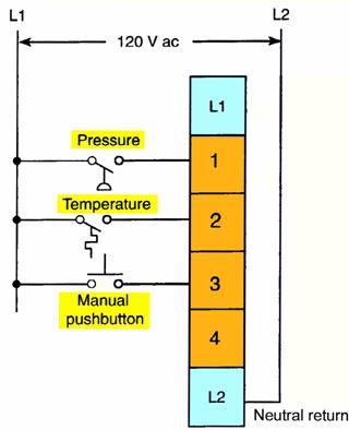
PLC Ladder Logic Program:

I/O address format will differ, depending on the PLC manufacturer. You give each input and output device an address. This lets the PLC know where they are physically connected. During each operating cycle, the controller examines the status of input devices, executes the user program, and changes outputs accordingly.The completion of one cycle of this sequence is called a scan. The scan time, the time required for one full cycle, provides a measure of the speed of response of the PLC Coil O/1 is energized when contacts I/1 and I/2 are closed or when contact I/3 is closed. Either of these conditions provides a continuous path from left to right across the rung that includes the coil.
Symbols:
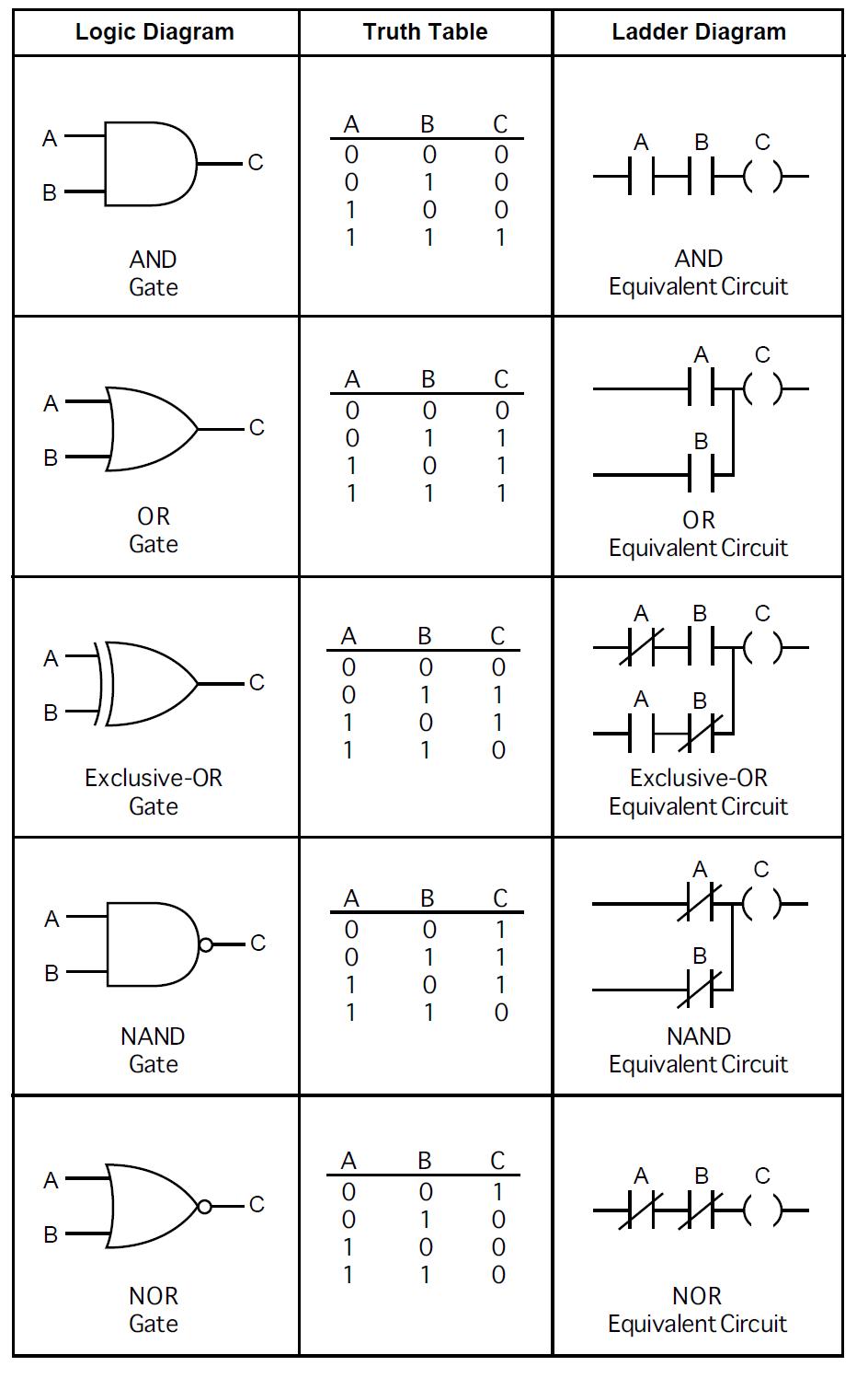
Introduction to Siemens PLC Step 7
STEP 7 is the basic programming and configuration software for SIMATIC. It is made up of a series of applications, each of which does a specific job within the scope of programming an automation task, such as:
Configuring and assigning parameters to the hardware
Creating and debugging user programs
Configuring networks and connections
The basic package can be extended by a range of optional packages, for example, additional programming language packages such as SCL, S7 Graph, or HiGraph.
The graphic user interface provided for these tasks is known as the SIMATIC Manager. The SIMATIC Manager collects all the data and the settings necessary for an automation task together in a project. Within this project the data are structured according to their function and represented as objects.
Objects:
In a similar way to the directory structure used in the Windows Explorer containing folders and files, a STEP 7 project is divided up into folders and objects. Objects which can contain other folders and objects are known as folders, for example, an S7 program which contains the folders "Blocks" and "Source files" and the object "Symbols."
Working with Objects:
The different types of object are linked directly in the SIMATIC Manager to the application in which they are required for processing. This means you do not have to remember which application you have to start in order to edit a specific object. You simply have to know what you have to do.
We recommend that you read the STEP 7 User Manual before you start work with STEP 7 to give yourself an overview of the basic principles, the variants, and the recommended procedures. If you are developing an S7 or M7 user program for the first time, the programming manuals Program Design for S7-300/S7-400 and for M7-300/M7-400 will provide the information you require about the structure and the elements of a user program.
Getting Started:
When you work with the SIMATIC Manager for the first time, you will find it useful to use the following procedure to help you get started. The description is based on programming in SIMATIC S7.
To create a new project and download it:
1. Create a new project with the help of the wizard you can open with the menu command File > "New Project" Wizard.
2. Double-click on the user program ("Blocks" object) that is contained in the folder "S7 program."
3. Now double-click on the OB1 displayed in the right half of the project window.
You can edit the block or create further blocks in the application started.
4. In the object properties of the S7 program, specify the MPI address for the module in which you want to test the blocks you have created. To do this, select the S7 program in the online view and select the menu command Edit > Object Properties.
5. In the offline view of the project window, select the user program ("Blocks" folder) or the blocks you want to download.
6. Download the selected objects to the programmable logic controller by selecting the menu command PLC > Download.
You can now debug the downloaded user program using the Monitor and Modify functions.
Objects and Object Hierarchy
In the same way that the Windows Explorer shows the directory structure of folders and files, the object hierarchy for projects and libraries in STEP 7 is shown in the SIMATIC Manager.
The following figure shows an example of an object hierarchy.
Objects have the following functions:
- Carriers of object properties,
- Folders,
- Carriers of functions (for example, to start a particular application).
Objects as Carriers of Properties
Objects can carry both functions and properties (such as settings). When you select an object, you can perform one of the following functions with it:
- Edit the object using the menu command Edit > Open Object.
- Open a dialog box using the menu command Edit > Object Properties and set object-specific options.
A folder can also be a carrier of properties.
Objects as Folders
A folder (directory) can contain other folders or objects. These are displayed when you open the folder.
Objects as Carriers of Functions
When you open an object, a window is displayed in which you can edit the object.
An object is either a folder or a carrier of functions. An exception to this is stations: they are both folders (for programmable modules) and carriers of functions (used to configure the hardware).
- If you double-click a station, the objects contained in it are displayed: the programmable modules and the station configuration (station as a folder).
- If you open a station with the menu command Edit > Open Object, you can configure this station and assign parameters to it (station as the carrier of a function). The menu command has the same effect as a double-click on the "Hardware" object.
Overview of STEP 7
What is STEP 7?
STEP 7 is the standard software package used for configuring and programming SIMATIC programmable logic controllers. It is part of the SIMATIC industry software. There are the following versions of the STEP 7 Standard package:
· STEP 7 Micro/DOS and STEP 7 Micro/Win for simpler stand-alone applications on the SIMATIC S7-200.
· STEP 7 for applications on SIMATIC S7-300/S7-400, SIMATIC M7-300/M7-400, and SIMATIC C7 with a wider range of functions
Can be extended as an option by the software products in the SIMATIC Industry Software (see also Extended Uses of the STEP 7 Standard Package) Opportunity of assigning parameters to function modules and communications processors. Forcing and multicomputing mode, Global data communication, Event-driven data transfer using communication function blocks, Configuring connections
Can be extended as an option by the software products in the SIMATIC Industry Software (see also Extended Uses of the STEP 7 Standard Package) Opportunity of assigning parameters to function modules and communications processors. Forcing and multicomputing mode, Global data communication, Event-driven data transfer using communication function blocks, Configuring connections
STEP 7 is the subject of this documentation, STEP 7 Micro is described in the "STEP 7 Micro/DOS" documentation.
Basic Tasks
When you create an automation solution with STEP 7, there are a series of basic tasks. The following figure shows the tasks that need to be performed for most projects and assigns them to a basic procedure. It refers you to the relevant chapter thus giving you the opportunity of moving through the manual to find task-related information.

Alternative Procedures:
As shown in the figure above, you have two alternative procedures:
- You can configure the hardware first and then program the blocks.
- You can, however, program the blocks first without configuring the hardware. This is recommended for service and maintenance work, for example, to integrate programmed blocks into in an existing project.
Brief Description of the Individual Steps:
- Install STEP 7 and license keys
- Plan your controller
- Design the program structure
Turn the tasks described in the draft of your controller design into a program structure using the blocks available in STEP 7 (see also Blocks in the User Program).
- Start STEP 7
- Create a project structure
A project is like a folder in which all data are stored in a hierarchical structure and are available to you at any time. After you have created a project, all other tasks are executed in this project (see also Project Structure).
- Configure a station
- Configure hardware
- Configure networks and communication connections
- Define symbols
- Create the program
- S7 only: generate and evaluate reference data
- Configure messages
- Configure operator control and monitoring variables
- Download programs to the programmable controller S7 only: after all configuration, parameter assignment, and programming tasks are completed, you can download your entire user program or individual blocks from it to the programmable controller (programmable module for your hardware solution). (See also Requirements for Downloading.) The CPU already contains the operating system.
· Test programsS7 only: for testing you can either display the values of variables from your user program or a CPU, assign values to the variables, or create a variable table for the variables that you want to display or modify (see also Introduction to Testing with the Variable Table). M7 only: test the user program with a high-level language-debugging tool.
· Monitor operation, diagnose hardwareYou determine the cause of a module fault by displaying online information about a module. You determine the causes for errors in user program processing with the help of the diagnostic buffer and the stack contents. You can also check whether a user program can run on a particular CPU (see also Hardware Diagnostics and Displaying Module Information).
· Document the plantAfter you have created a project/plant, it makes sense to produce clear documentation of the project data to make further editing of the project and any service activities easier (see also Printing Project Documentation). DOCPRO, the optional tool for creating and managing plant documentation, allows you to structure the project data, put it into wiring manual form, and print it out in a common format.
Specialized Topics
When you create an automation solution there are a number of special topics that may be of interest to you:
· Multicomputing - Synchronous Operation of Several CPUs (see also Multicomputing - Synchronous Operation of Several CPUs)
· More than One User Working in a Project (see also More than One User Editing Projects)
· Working with M7 Systems (see also Procedure for M7 Systems)
Project Structure
Projects are used to store the data and programs which are created when you put together an automation solution. The data collected together in a project include:
- Configuration data on the hardware structure and parameters for modules,
- Configuration data for communication in networks, and
- Programs for programmable modules.
The main task when you create a project is preparing these data for programming.
Data are stored in a project in object form. The objects in a project are arranged in a tree structure (project hierarchy). The display of the hierarchy in the project window is similar to that of the Windows Explorer. Only the object icons have a different appearance.
The top end of the project hierarchy is structured as follows:
- 1st Level: Project
- 2nd Level: Subnets, stations, or S7/M7 programs
- 3rd Level: depends on the object in level 2.
Project Window
The project window is split into two halves. The left half shows the tree structure of the project. The right half shows the objects that are contained in the object open in the left half in the selected view (large symbols, small symbols, list, or details).
Click in the left half of the window on the box containing a plus sign to display the full tree structure of the project. The resulting structure will look something like the following figure.

At the top of the object hierarchy is the object "S7_Pro1" as the icon for the whole project. It can be used to display the project properties and serves as a folder for networks (for configuring networks), stations (for configuring the hardware), and for S7 or M7 programs (for creating software). The objects in the project are displayed in the right half of the project window when you select the project icon. The objects at the top of this type of object hierarchy (libraries as well as projects) form the starting point in dialog boxes used to select objects.
Project View

You can display the project structure for the data available on the programming device in the component view "offline" and for the data available on the programmable control system in the component view "online" in project windows.
An additional view you can set is available if the respective optional package is installed: the plant view.
Note: Configuring hardware and networks can only be done in the "offline" view.
|
Library Object
A library can contain S7/M7 programs and is used to store blocks. A library is located at the top of an object hierarchy.
 |
|
Symbol
|
Object Folder
|
Selection of Important Functions
|
Library
|
Symbol
|
Objects in the Library Level
|
Selection of Important Functions
|
S7 program
M7 program
|
|
How to Set Up Projects
To create a project with the wizard, proceed as follows:
1. Select the menu command File > "New Project" Wizard in the SIMATIC Manager.
2. Enter the details required by the wizard in the dialog boxes.
To create a project manually, proceed as follows:
1. Select the menu command File > New in the SIMATIC Manager.
2. In the "New" dialog box select the option "User Projects".
3. Make sure you have selected the entry "Project" in the "Type:" dropdown list.
4. Click on the check box "Insert in current multiproject" to insert the project in a multiproject. You can only enable the checkbox after you have selected the multiproject in the project window.
5. Enter the name of the new user project in the "Name:" box. You can also select a name from the list above and modifiy it to form the new project name.
6. Create the new user project and confirm your entries with "OK".
To copy a project, proceed as follows:
1. Select the project you want to copy.
2. Select the menu command File > Save As in the SIMATIC Manager.
3. Decide in the "Save As" dialog box whether you want to rearrange before saving or not. With older projects or projects in which you have made a lot of changes, you should select the option "Rearrange before saving" so that the data storage is optimized and the project structure checked.
4. In the "Save Project As" dialog box, enter the name of the new project and a new storage path if necessary. Confirm with "OK."
If you want to copy a part of a project such as stations, software, blocks, etc., proceed as follows:
1. Select the part of the project you want to copy.
2. Select the menu command Edit > Copy in the SIMATIC Manager.
3. Select the folder in which the copied part of the project is to be stored.
4. Select the menu command Edit > Paste.
To delete a project, proceed as follows:
1. Select the menu command File > Delete in the SIMATIC Manager.
2. In the "Delete" dialog box, activate the option button "Project." The projects are listed in the list box below it.
3. Select the part of the project you want to delete and confirm with "OK."
4. Confirm the prompt with "Yes."
To delete part of a project, proceed as follows:
1. Select the part of the project you want to delete.
2. Select the menu command Edit > Delete in the SIMATIC Manager.
3. Confirm the prompt with "Yes."
To create a new station in a project, open the project so that the project window is displayed.
1. Select the project.
2. Create the object "Station" for the required hardware by using the menu command Insert > Station.
Click on the "+" sign in front of the project icon in the project window if the station is not displayed.
To configure the hardware, proceed as follows:
1. Click on the new station. It contains the "Hardware" object.
2. Open the "Hardware" object. The "Hardware Configuration" window is displayed.
3. In the "Hardware Configuration" window, plan the structure of the station. A module catalog is available to help you. You open the catalog using the menu command View > Catalog.
4. First, insert a rack from the module catalog in the empty window. Then select the modules and place them in the rack slots. At least one CPU must be configured per station.
If these objects are not yet visible in the project window, click the "+" in front of the station icon in the project window to display the module and click the box in front of the module to display the S7/M7 program and the "Connections" object.
To create the software for your project, proceed as follows:
1. Open the S7 program or M7 program.
2. Open the "Symbols" object in the S7 or M7 program and assign the symbols. (This step can also be done later.)
3. Open the "Blocks" folder if you want to create blocks or the "Source Files" folder if you want to create a source file.
4. Insert a block or a source file. The menu commands for this are:
§ Insert > S7 Block
§ Insert > S7 Software
§ Insert > M7 Software
5. Open the block or the source file and enter a program. You will find more information on programs in the programming language manuals.
6. Document the project using the menu command Insert > Project Documentation.To document a STEP 7 project you can organize all the configuration data created with STEP 7 in wiring manuals. This function is only available if the "DOCPRO" optional package is installed.
Depending on your task, you may not need to perform all these steps.
Creating and Managing Objects
Some basic processing steps are the same for all objects and do not depend on the object type. These standard handling sequences are summarized here. This knowledge of standard procedures is required to move on to other sections in the manual.
The usual sequence of steps when handling objects is:
- Create an object
- Select an object
- Perform actions with the object (for example, copy, delete).
Setting the Path to Create New Projects/Libraries
New user projects, libraries and multiprojects are stored in the default folder "\Siemens\Step7\S7proj". If you want to store them in another folder, you should set your custom path for these objects before you save projects, libraries and multiprojects for the first time. To do this, select the menu command Options > Customize. In the "General" tab of the dialog box displayed you can specify the path name under which you want to store new projects or libraries.
Creating Objects
The STEP 7 wizard "New Project" offers support with creating a new project and inserting objects. Use the menu command File > "New Project" Wizard to open the wizard. In the dialog boxes displayed you can set the structure of your project and then have the wizard create the project for you.
If you do not wish to use the wizard, you can create projects and libraries using the menu command File > New. These objects form the starting point of an object hierarchy. You can create all other objects in the hierarchy using the commands in the Insert menu, provided they are not created automatically. The exception to this are the modules in a SIMATIC station which are created when you configure the hardware or by using the "New Project" wizard.
Opening Objects
There are a number of ways to open an object in the detailed view:
- Double-click on the object icon
- Select the object and then the menu command Edit > Open Object. This only works for objects that are not folders.
Once you have opened an object, you can create or change its contents.
When you open an object that does not contain other objects, its contents are represented by a suitable software component in a new window for editing purposes. You cannot change objects whose contents are already being used elsewhere.
Note
Exception: Stations appear as folders for programmable modules (when you double-click them) and for the station configuration. If you double-click the "Hardware" object, the application for configuring hardware is started. Selecting the station and selecting the menu command Edit > Open Object has the same effect.
|
Building an Object Hierarchy
Use the "New Project" wizard to create the object hierarchy. When you open a folder, the objects it contains are displayed on the screen. You can now create more objects in the folder using the Insert menu, for example, additional stations in a project. Only the commands for those objects which can be inserted in the current folder are active in the Insert menu.
Setting Object Properties
Object properties are data belonging to the object which determine its behavior. The dialog box for setting object properties appears automatically when you create a new object and properties have to be set. The properties can also be changed at a later date.
Using the menu command Edit > Object Properties, a dialog box is opened in which you can display or set the properties for the selected object.
Using the menu command Edit > Special Object Properties, you can open dialog boxes and enter data required for operator control and monitoring functions and for configuring messages.
For example, in order to display the special object properties of a block for operator control and monitoring, the block must be marked as being relevant for operator control and monitoring, meaning that the system attribute "s7_m_c" must be set to the value "true" in the "Attributes" tab of the block properties.
Note:
|
Properties of the "System Data" folder and the "Hardware" object cannot be displayed or changed.You cannot write in the dialog boxes for object properties of a read-only project.In this case, the input boxes are grayed out.If you display the properties of programmable modules, you cannot edit the displayed parameters for reasons of consistency. To edit the parameters you must open the "Configuring Hardware" application. If you change the settings for objects on the programming device (for example, the configuration data of a module), they are not yet effective in the target system, because the system data blocks in which the settings are saved have to be in the target system. If you load an entire user program, the system data blocks are also automatically transferred. If you change the settings after having loaded the program, you can reload the "System data" object in order to transfer the settings to the target system. It is strongly recommended to edit the folders exclusively with STEP 7, since they can be physically structured in a different way than you see in the SIMATIC Manager.Cutting, Pasting, Copying
Most objects can be cut, pasted, or copied as usual under Windows. The menu commands for these functions are found in the Edit menu.
You can also copy objects by dragging and dropping. If you attempt to move or copy to an illegal destination, the cursor displays a prohibited sign as a warning.
When you copy an object, the whole hierarchy beneath it is also copied. This enables components you create in an automation task to be used again and again.
NoteThe connection table in the "Connections" folder cannot be copied. Note that when you copy lists of operator-relevant texts, only those languages installed in the destination object are accepted.
Renaming Objects
The SIMATIC Manager assigns standard names to some new objects. These names are generally formed from the type of object (if a number of objects of this type can be created in the same folder) and a number.
For example, the first S7 program will be named "S7 Program(1)", the second "S7 Program(2)" etc. The symbol table is simply called "Symbols" as it can only exist once in each folder.
You can change the names of most objects and assign them names which are more relevant to their content.
With projects, the directory names in the path must not have more than 8 characters. Otherwise, there may be problems when archiving and using "C for M7" (Borland compiler).
You can change the name of an object directly or using the object properties.
Directly:
When you slowly click twice on the name of a selected object, a frame appears around the text. You can then edit the name using the keyboard.
Using the menu:
Select the required object in the project window and select the menu command Edit > Rename. A frame appears around the text. You can then edit the name using the keyboard.
If you are not allowed to change the name:
If you are not allowed to change the name of an object, the input field is shown in gray in the dialog box, the current name is displayed, and text entries are not possible.
You will find a step-by-step guide to renaming under Renaming Objects. Note If you move the mouse pointer out of the name box while editing the name and execute another action (for example, select a menu command), the edit procedure is terminated. The changed name is accepted and entered if it is allowed.
Moving Objects
With the SIMATIC Manager you can move objects from one folder to another even if the destination is in another project. When you move a folder its contents are all moved as well.
Note
You cannot move the following objects:
|
You will find a step-by-step guide to moving under Moving Objects.
Sorting Objects
You can sort objects in the detailed view (menu command View > Details) according to their attributes. To do this, click on the corresponding header of the required attribute. When you click again, the sort order is reversed. Blocks of one type are sorted according to their numerical order, for example, FB1, FB2, FB11, FB12, FB21, FC1.
Default Sort Order
When you re-open a project, the objects in the detailed view are displayed according to a default sort order. Examples:
- Blocks are shown in the order "System data, OB, FB, FC, DB, DUTY, VAT, SFB, SFC."
- In a project, all stations are shown first and then the S7 programs.
The default is not therefore an alphanumeric ascending or descending sort order in the detailed view.
Restoring the Default Sort Order
After resorting, for example, by clicking on the column header "Object Name," you can restore the default order if you proceed as follows:
- Click the column header "Type" in the detailed view.
- Close the project and open it again.
Deleting Objects
You can delete folders and objects. If you delete a folder, all the objects contained in it are also deleted.
You cannot undo the delete procedure. If you are not sure whether you really no longer need an object, it is better to archive the whole project first.
Note
You cannot delete the following objects:
|
You will find a step-by-step guide to deleting under Deleting Objects.
Overview: Procedure for Configuring and Assigning Parameters to a Local Configuration
Requirement
You must have opened a project or created a new project in the SIMATIC Manager.
Basic Procedure
To configure and assign parameters to a structure, proceed as shown below:

Creating a Station
Requirement
You must have opened the SIMATIC Manager and opened a project or created a new project.
Procedure
A station can only be created directly beneath a project.
1. Select the project in the left half of the project window.
2. Select the menu command Insert > Station > SIMATIC 300-Station or ... > SIMATIC 400-Station.
The station is created with a preset name. You can replace the name of the station with a more relevant name of your own.
The station is created with a preset name. You can replace the name of the station with a more relevant name of your own.
Starting the Application to Configure the Hardware
Requirement
You must have created a station (SIMATIC 300, SIMATIC 400).
Procedure
- Select the "Station" object in the project window so that the "Hardware" object becomes visible in the right half of the station window.
§ "Station" object
|
- Double click on the "Hardware" object.
§ "Hardware" object
|
§ Alternatively you can select the "Station" object and then the menu command Edit > Open Object.
§ Result: A station window and the module catalog (if it was still open when you last exited the application) appear on the screen. You can position racks and other components in accordance with the station structure; select the components required for the station structure from the module catalog ("Hardware Catalog" window).
Opening More Stations
Using the menu command Station > New you can configure another station in the same project; using Station > Open you can open an existing (offline) station configuration for editing.
Arranging the Central Rack
Requirement
The station window must be open and you must have a plan of the hardware configuration of the station.
Procedure
1. Select a suitable central rack ("Rack") for your configuration from the "Hardware Catalog" window; in SIMATIC 300 the Rail, in SIMATIC 400 the Universal rack (UR1), for example.
2. Drag the rack to the station window.
The rack appears in the form of a small configuration table in the upper part of the station window. In the lower part of the window, the detailed view of the rack appears with additional information such as the order number, MPI address, and I/O addresses. Alternatively to steps 1 and 2, you can also double-click the rack in the "Hardware Catalog" window.
The rack appears in the form of a small configuration table in the upper part of the station window. In the lower part of the window, the detailed view of the rack appears with additional information such as the order number, MPI address, and I/O addresses. Alternatively to steps 1 and 2, you can also double-click the rack in the "Hardware Catalog" window.
Arranging Modules in a Rack
Requirements
You have arranged a rack in a station window and the rack is not shown minimized (the rack slots are visible).
If you want to have the visual advantage of having the available slots of a selected module highlighted in color in STEP 7, your monitor display must set for more than 256 colors.
Procedure
- Select a module (for example, a CPU) from the "Hardware Catalog" window.The slots available for this module are highlighted in color.
- Drag & drop the module into the appropriate row of the rack (configuration table). STEP 7 checks whether any slot rules are violated (an S7-300 CPU must not, for example, be inserted in slot 2).
- Repeat steps 1 and 2 until the rack has been fully equipped with the required modules.
Alternatively, you can also select the appropriate row in the configuration table and double-click on the required module in the "Hardware Catalog" window.
If no row in the rack is selected and you double-click a module in the "Hardware Catalog" window, the module will then be placed in the first available slot.
Tip
After you have selected a slot of a module rack, you can open the context-sensitive menu (right-click) Insert Object or Replace Object to view a list of modules you can insert. This feature saves you the search through the Hardware Catalog. You select from all the modules that are listed in the currently available catalog profile.
Display of Interfaces and Interface Sub modules
The interfaces and interface submodules are shown in the configuration table in a separate row. The row has the same name as the interface (for example, X1) or - if the module has slots for interface submodules - bears the prefix "IF" (for example, IF1).
With integrated interfaces the name of the interface appears in the "Module" column; with modules with slots for interface submodules you can copy a suitable interface submodule (IF) from the "Hardware Catalog" window to the appropriate row using drag & drop.
Assigning Properties to Modules/Interfaces
Introduction
Properties of components such as modules or interfaces are addresses and parameters. Only if you want to change the default values do you need to read the following sections.
Requirement
You have arranged in the configuration table the component for which you want to modify the properties.
Procedure
Every component (module, interface, or interface submodule) has default properties; for example, default measurement types and measuring ranges for analog input modules.
If you want to change these settings, proceed as follows:
1. Double-click in the configuration table on the component (for example, module or interface submodule) that is to have parameters assigned or select the row and select the Edit > Object Properties menu command.Using the right-hand mouse button: Move the mouse pointer to the component, press the right-hand mouse button, and select the Object Properties command from the pop-up menu
2. Use the displayed tabbed dialog boxes to assign the component properties.
Saving a Configuration and Checking the Consistency
To save a configuration with all set parameters and addresses, select the menu command Station > Save or Station > Save and Compile.
If you use the menu command Station > Save and Compile, the configuration is saved in the active project as a "Station" object and if valid system data blocks (SDB) could be created, they are stored in the (offline) "Blocks" folder for the associated modules ("SDB carrier," for example, CPU). The system data blocks are represented by the "System Data" folder/symbol.
Symbol for system data
|
To be able to save incomplete configurations, select the menu command Station > Save. Using this command no system data blocks are created when saving. The save procedure takes less time than if you save and compile, but you should be aware that there may be inconsistencies between the configuration saved in the "Station" object and the configuration saved in the system data.
Before downloading, you should check your station configuration for errors using the menu command Station > Consistency Check.
Downloading a Configuration to a Programmable Controller
Tip
Before downloading, use the Station > Check Consistency menu command to make sure there are no errors in your station configuration. STEP 7 then checks to see whether downloadable system data can be created from the present configuration. Any errors found during consistency checking are displayed in a window.
Requirements for Downloading
- The programming device (PG) is connected to the MPI interface of the CPU using an MPI cable.
- In a networked system (programming device is connected to a subnet):All modules in a subnet must have different node addresses and the actual configuration must match the network configuration you created.
- The present configuration must match the actual station structure.A configuration can only be downloaded to the station if it is consistent and free of errors. Only then can system data blocks (SDBs) be created which can in turn be downloaded to the modules.
- If the station structure contains modules that were configured and assigned parameters using optional software packages: The optional package must be authorized.
Procedure
- Select the menu command PLC > Download To Module. STEP 7 guides you by means of dialog boxes to the result.
The configuration for the complete programmable controller is downloaded to the CPU. The CPU parameters become active immediately. The parameters for the other modules are transferred to the modules during startup.
Note
Partial configurations, for example, the configuration of individual racks, cannot be downloaded to a station. For consistency reasons, STEP 7 always downloads the whole configuration to the station.
|
Changing the CPU Operating Mode During Downloading
When you trigger the function PLC > Download, you can execute the following actions on the programming device guided by the dialog boxes:
- Switch the CPU to STOP(if the mode selector is set to RUNP or the connection to the CPU is authorized by password)
- Compress the memory(if not enough continuous free memory is available)
- Switch the CPU back to RUN
Uploading from the Programmable Controller to the PG/PC
This function supports you when carrying out the following actions:
- Saving information from the programmable controller (for example, for servicing purposes)
- Fast configuring and editing of a station, if the hardware components are available before you start configuring.
Saving Information from the Programmable Controller
This measure may be necessary if, for example, the offline project data of the version running on the CPU are not, or only partially, available. In this case, you can at least retrieve the project data that are available online and upload them to your programming device.
Fast Configuring
Entering the station configuration is easier if you upload the configuration data from the programmable controller to your programming device after you have configured the hardware and restarted (warm restart) the station. This provides you with the station configuration and the types of the individual modules. Then all you have to do is specify these modules in more detail (order number) and assign them parameters.
The following information is uploaded to the programming device:
- S7-300: Configuration for the central rack and any expansion racks
- S7-400: Configuration of the central rack with a CPU and signal modules without expansion racks
- Configuration data for the distributed I/O cannot be uploaded to the programming device.
This information is uploaded if there is no configuration information on the programmable controller; for example, if a memory reset has been carried out on the system. Otherwise, the Upload function provides much better results.
For S7-300 systems without distributed I/O, all you have to do is specify these modules in more detail (order number) and assign them parameters.
Note
When you upload data (if you do not already have an offline configuration), STEP 7 cannot determine all the order numbers of the components.
You can enter the "incomplete" order numbers when you configure the hardware using the menu command Options > Specify Module. In this way, you can assign parameters to modules that STEP 7 does not recognize (that is, modules that do not appear in the "Hardware Catalog" window); however, STEP 7 will not then check whether you are keeping to the parameter rules.
|
Restrictions when Uploading from the Programmable Controller
The following restrictions apply to the data uploaded from the programmable controller to the programming device:
- Blocks do not contain any symbolic names for parameters, variables, and labels
- Blocks do not contain any comments
- The entire program is uploaded with all the system data, whereby the system can only continue to process the system data belonging to the "Configuring Hardware" application
- The data for global data communication (GD) and configuring symbol-related messages cannot be processed further
- Force jobs are not uploaded to the programming device with the other data. They must be saved separately as a variable table (VAT)
- Comments in the module dialog boxes are not uploaded
- The names of the modules are only displayed if this option has been selected during configuration (HW Config: the option "Save object names in the programmable logic controller" in the dialog box under Options > Customize).
Basic Procedure for Configuring a DP Master System
If you know the principles of how to configure a central structure, you also know how to configure the distributed I/O - the procedure is the same to a large extent.
Station Window as an Image of the Real DP Master System
When you place a DP master (for example, a CPU 315-2DP), STEP 7 automatically draws a line that represents the master system. At the end of the line, place the DP slaves that are assigned to this DP master using drag & drop from the "Hardware Catalog" window under "PROFIBUS-DP."
As a DP master system is always connected to a PROFIBUS subnet, STEP 7 automatically displays dialog boxes for setting the subnet properties (for example, transmission rate) and the PROFIBUS address when you place the DP components.
DP Slave Does Not Appear in the "Hardware Catalog" Window
If a DP slave does not appear in the "Hardware Catalog" window, you must install the corresponding *.GSD file after the start of STEP 7 using the menu command Options > Install GSD File. The dialog boxes then guide you through the process of installing the *.GSD file. The installed DP slave then appears in the "Hardware Catalog" window under "PROFIBUS-DP - Other Field Devices."

Slave Configuration in the Detailed View
If you select the DP slave, the slave structure (DP identifiers and modules/submodules) and I/O addresses are displayed in the detailed view of the station window.
Switching Between the DP Master System and the DP Slave in the Detailed View of the Station Window
If you select the symbol for the DP master system , all DP slaves belonging to the DP master system will be displayed in the lower half of the station window. If you select a DP slave symbol, the configuration of the DP slave is displayed in the lower half of the station window. You can easily change between displays by using the following buttons:
and Slot Numbering in Distributed I/O Devices. Depending on which DP slave type you are configuring, the slots in the detailed view of the DP slave begin either with "0" or "4."
and Slot Numbering in Distributed I/O Devices. Depending on which DP slave type you are configuring, the slots in the detailed view of the DP slave begin either with "0" or "4."
With DP slaves that are configured by *.GSD files, the *.GSD file specifies at which slot the I/O addresses start; the slots before that are "empty."
Slot numbering of DP slaves such as ET 200M that are completely integrated in STEP 7 is derived from the structure of an S7-300 station according to the following pattern:

Remarks on the slots of a DP slave, which is structured like the S7-300 station:
· The "actual" I/O (inputs/outputs) always starts with slot 4.
· Independent of whether a power supply module (PS) is inserted in the real configuration or not: slot 1 is always reserved for a PS.
· Slot 2 is always reserved for the DP interface module.
· Slot 3 is always reserved for an expansion interface module (IM), independent of whether a "real" I/O device can be expanded or not.
This pattern is used for all DP slave types: modular and compact. The slot arrangement is important for evaluating diagnostic messages (the slot that triggers diagnostics).
Tips for Editing Station Configurations
Docking the "Hardware Catalog" Window on the Side of the Station Window
To prevent the "Hardware Catalog" window obscuring the contents of the station window, you can "dock" it on one side edge of the station window; meaning it is then positioned and fixed there. Simply double-click the area above the "Profile" list box in the Hardware Catalog. To release the "docked" window, double-click in this area once again.
You can change the size (height and width) of the "Hardware Catalog" window when the window is undocked. When the window is docked, the width of the "Hardware Catalog" window can be changed.
Recognizing Available Slots
As of STEP 7 V5.2 you can easy recognize available slots for modules at first glance, provided your monitor display is set to more than 256 colors. If you select a module in the hardware catalog and the module can be inserted in a configured rack, then the possible slots for this module are highlighted in color. This feature makes configuration faster and easier for you.
If you click a module in the "Hardware Catalog" window, and no slot is selected, the module will then be placed in the first available slot.
Selecting a Number of Rows in the Configuration Table
If you want to select a number of rows in the configuration table to copy (for example, using the pop-up menu command Copy) or delete (for example, using the pop-up menu command Delete) a number of modules or insert a number of modules of the same type, proceed as follows:
To select all rows:
|
Select the menu command Edit > Select > All.
|
To select a group of consecutive rows:
|
Click on the first row of the group you want to select.
Keep the SHIFT key pressed and click on the last row of the group you want to select.
|
To select a number of rows:
|
Press CTRL, keep it pressed, and click on each row you want to select.
|
You can also insert copied modules beyond the limitations of stations if you do not violate any slot rules when inserting.
Handling Complex Stations
If you have a complex station structure with a lot of racks, for example, you can set the configuration tables to their minimum size.
- Select the configuration table.
- Press the right mouse button and select the menu command Minimize in the popup menu.
You can also set this overview using the menu command Options > Customize.
Arranging the Racks in the View Automatically
Using the menu command View > Arrange Automatically you can let STEP 7 arrange your current view automatically.
Displaying Insertable ("Pluggable") Components in the Hardware Catalog
If you have selected a slot in a rack, then you can use the menu commands Insert > Insert Object or Insert > Change Object to display a selection of modules than can be inserted. This method saves you from having to search through the hardware catalog. You can select from all modules that are available in the current catalog profile.
Multicomputing - Synchronous Operation of Several CPUs
What is Multicomputing Operation?
Multicomputing means the simultaneous operation of more than one CPU with multicomputing capability (up to a maximum of four) in one central rack of the S7-400.
The participating CPUs automatically change their operating modes synchronously, meaning the CPUs start up together and go into STOP mode together. The user program for each CPU executes independently of the user programs in the other CPUs. This means control tasks can be run in parallel.
Example
The following figure shows a programmable controller that will operate in multicomputing mode. Each CPU can access the modules assigned to it (FM, CP, SM).

Difference Between Multicomputing and Operation in Segmented Racks
Simultaneous unsynchronized operation of more than one CPU in a segmented rack CR2 (physically segmented, cannot be set by user) is also possible. This is, however, not multicomputing. The CPUs in a segmented rack form their own independent subsystem and behave like single processors. There is no shared address area.
"Multicomputing mode" and "unsynchronized operation in a segmented rack" at the same time is not possible.
Slot Rules
In multicomputing mode up to four CPUs can be inserted simultaneously in a central rack in any order.
If you use CPUs that can manage only module start addresses that are divisible by four (generally CPUs before 10/98), you must follow this rule for all configured CPUs when you assign the addresses. The rule applies to a case where you are also using CPUs that permit byte-by-byte assignment of module start addresses in single-computing operation.
Bus Connection
The CPUs are interconnected via the communication bus (corresponds to a connection via MPI).
Behavior During Startup and Operation
During startup the CPUs in multicomputing operation check automatically whether they can synchronize. Synchronization is only possible:
· If all (and only) the configured CPUs are inserted and not defective
· If correct configuration data (SDBs) were created and downloaded for all inserted CPUs.If one of these prerequisites is not met, the event is entered in the diagnostic buffer under the ID 0x49A4. You will find explanations of the event IDs in the reference online help on standard and system functions (SFBs/SFCs).
When the CPUs exit STOP mode, the startup types are compared (COLD RESTART/WARM RESTART/HOT RESTART). This ensures that all the CPUs in the programmable controller execute the same type of startup and all CPUs have the same operating mode.
Address and Interrupt Assignment
In multicomputing mode the individual CPUs can access the modules assigned to them during configuration with STEP 7. The address area of a module is always exclusively assigned to a CPU.
All CPUs share the same address space; this means that the logical address of a module is only present once in the multi-computing station.
An interrupt input is assigned to every CPU. Interrupts received at this input cannot be received by the other CPUs. The assignment of the interrupt line is made automatically during parameter assignment of the modules.
The following rules apply to interrupt servicing:
· Hardware interrupts and diagnostic interrupts are sent to only one CPU.
· If there is a module failure, the interrupt is serviced by the CPU to which the module was assigned with STEP 7.
· When a CP is inserted or removed and the "Address setting for LOCK/UNLOCK with FETCH/WRITE, SPEED Send/Receive" check box exists in the "Addresses" tab of the Properties dialog, then the following applies:
§ If the check box is selected, a remove/insert interrupt is reported only on the assigned CPU and OB83 is started.
§ If the check box is not selected, a remove/insert interrupt is reported all CPUs and OB83 is started.
· If a rack fails, OB86 is called on every CPU.
You will find more detailed information on OB86 in the reference online help on organization blocks.
Multicomputing has advantages in the following situations:
· When your user program is too large for one CPU and memory is used up, distribute your program among more than one CPU.
· If part of your system must be processed quickly, take these program sections out of the main program and run them on a separate fast CPU.
· If your system consists of various parts that can be clearly delineated and can be controlled relatively autonomously, run the program for system section 1 on CPU 1 and system section 2 on CPU 2 etc.
Setting Multicomputing Operation
Multicomputing operation results implicitly when you insert a second (third or fourth) multicomputing CPU in a rack suitable for this kind of operation (for example, the rack UR1). When a module is selected, the info text in the "Hardware Catalog" window tells you whether the CPU has multicomputing capability.
Requirements
Before you can configure modules in your programmable controller for multicomputing mode, the following conditions must be satisfied:
· You must have set up your programmable controller as described in the "S7-400, M7-400 Programmable Controllers, Hardware and Installation" manual.
· You must have opened the configuration table in the project window by double-clicking the "Hardware" object.
· You must have arranged a rack in the station window and the rack is shown as being open (the rack slots are visible).
Basic Procedure

Note when Downloading and Uploading
Only the complete station configuration should be downloaded to all CPUs. This avoids inconsistent configurations.
When uploading to a programming device, the station configuration is loaded from all programmable modules, one after another (CPU by CPU). You have the option of aborting the upload process even if not all the configuration data (SDBs) were uploaded. In this case, parameter assignment information will be lost.
Programming
Programming for the multicomputing mode is essentially the same as programming a single CPU.
Extra steps are, however, necessary if you want to synchronize the CPUs so that they react to events together.
Calling SFC35
If you want all the CPUs to react to events (for example, interrupts) together in the multicomputing mode, you program an SFC35 "MP_ALM" call. Calling SFC35 triggers a multicomputing interrupt that causes a synchronized request for OB60 on all CPUs. This OB contains local variables that specify the triggering event in greater detail.
When SFC35 is called, the information about the events is transferred to all CPUs in a job identifier. The job identifier allows 16 different events to be distinguished.
When they service the multicomputing interrupt, both the sending user program and the user programs on the other CPUs check whether or not they recognize the job and then react as programmed.
You can call SFC35 at any point in your program. Since the call is only of practical use in RUN mode, the multicomputing interrupt is suppressed if it is triggered in STARTUP mode.
The multicomputing interrupt can only be triggered again after the current multicomputing interrupt has been serviced (acknowledged).
You will find more detailed information on SFC35 in the reference online help on SFBs/SFCs.
Programming OB60
You can program a specific OB60 for each separate CPU and download it to the CPU. This means that the execution times can differ from CPU to CPU. This leads to the following behavior:
· The interrupted priority classes on the CPUs are continued at different times.
· A multicomputing interrupt is not serviced if it occurs during the execution of OB60 on any of the CPUs. A message is, however, generated and you can check this and react accordingly.
If OB60 is not loaded on one of the CPUs, this CPU returns immediately to the last priority class and continues the program there.
You will find more detailed information on OB86 in the reference online help on organization blocks.
Networking Stations within a Project
Context: Network Configuration and STEP 7 Projects
Subnets lie directly beneath a project in the object hierarchy and can therefore only be managed within a project. You can, however, connect nodes together that were configured in different projects.
If possible, you should create and configure nodes that you want to connect in networks in the same project.
Subnets and Stations
You can create the subnets and stations in a STEP 7 project and then configure the stations for communication very easily.
As a result of the different tasks of the stations or the fact that the plant has increased in size and scope, it may be necessary to run a number of subnets. These subnets can also be managed in one project. A station can be assigned to a number of subnets by assigning the communication nodes (for example, CPs) accordingly.

Basic Procedure for Creating Logic Blocks
Logic blocks (OBs, FBs, FCs) consist of a variable declaration section, a code section as well as their properties. When programming, you must edit the following three parts:
- Variable declaration: In the variable declaration you specify the parameters, system attributes for parameters, and local block-specific variables.
- Code section: In the code section you program the block code to be processed by the programmable controller. This consists of one or more networks. To create networks you can use, for example, the programming languages Ladder Logic (LAD), Function Block Diagram (FBD), or Statement List (STL).
- Block properties: The block properties contain additional information such as a time stamp or path that is entered by the system. In addition, you can enter your own details such as name, family, version, and author and you can assign system attributes for blocks.
In principle it does not matter in which order you edit the parts of a logic block. You can, of course, also correct them and add to them.

Note
If you want to make use of symbols in the symbol table, you should first check that they are complete and make any necessary corrections.
|
Configuring Messages
Messages allow you to detect, localize, and remedy errors during processing on the programmable controllers quickly, thus reducing downtimes on a plant considerably.
Before messages can be output, they must first be configured.
With STEP 7, you can create and edit messages linked to events with assigned message texts and message attributes. You can also compile the messages and display them on display devices.
Block-related messages are assigned to a block (instance DB). To create a block-related message, you can use system function blocks (SFBs) and system functions (SFCs) as message blocks
Basic Procedure

Programming Message-Type Blocks (FB)
- In the SIMATIC Manager select the function block (FB) for which you want to generate a block-related message and open this block with a double-click.Result: The selected block is opened and displayed in the "LAD/STL/FBD" window.
- Fill out the variable declaration table. For every message block that is called in the function block you must declare variables in the calling function block.Enter the following variables in the variable overview column:
- For the parameter "IN" enter a symbolic name for the message block input, for example, "Meld01" (for message input 01) and the data type (must be "DWORD" without an initial value).
- For the parameter "STAT" enter a symbolic name for the message block to be called, for example, "alarm" and the corresponding data type, in this case "SFB33."
- In the code section of the function block, insert the call for the selected message block, here "CALL alarm", and finish your entry with RETURN.Result: The input variables for the called message block (here SFB33) are displayed in the code section of the function block.
- Assign the symbolic name you assigned in step 2 for the message block input, here "Mess01," to the variable "EV_ID". The system attributes are now applied for the message of type "alarm".Result: A flag should appear in the "Name" column for the parameter "IN" if the column is not selected. The selected block is then set as a message-type block. The required system attributes (for example, S7_server and S7_a_type) and the corresponding values are assigned automatically (Note: for certain SFCs you will have to assign the system attributes for the parameter "IN" yourself. To do this select the menu command Edit > Object Properties and then select the "Attributes" tab.).Caution: If you do not call an SFB, but rather an FB that contains multiple instances and configured messages, you must also configure the messages of this FB, with multiple instances, in the calling block.
- Repeat steps 2 to 4 for all calls to message blocks in this function block.
- Save the block using the menu command File > Save.
- Close the "LAD/STL/FBD" window.
Opening the Message Configuration Dialog Box
- Select the desired message block and then select the menu command Edit > Special Object Properties > Message in the SIMATIC Manager.Result: The STEP 7 message configuration dialog box (standard dialog box) is opened. Information on opening the PCS7 Message Configuration function can be found under PCS 7 Message Configuration.
Editing a Message Type
- Select the desired message block, open the message configuration, and enter the required message text in the "Text" and "Attributes" tabs or select the required message attributes.If you selected a multi-channel message block (for example, "ALARM_8"), you can assign specific texts and, to certain extent, specific attributes to each subnumber.
- Assign the required display devices to the message type by clicking the "New Device" button and selecting the required display devices in the "Add Display Device" dialog box.
In the following tabbed pages, enter the required texts and attributes for the display devices. Exit the dialog box with "OK".
Note
When editing the display device specific texts and attributes, please read the documentation supplied with your display device.
|
Creating Instance Data Blocks
- When you have created a message type, you can associate instance data blocks to it and edit the instance-specific messages for these data blocks.To do this, in the SIMATIC Manager open the block that is to call your previously configured function block, for example, "OB1", by double-clicking it. In the open code section of the OB, enter the call ("CALL"), the name and number of the FB to be called and of the instance DB that you want to associate with the FB as an instance. Confirm your entry with RETURN. Example: Enter "CALL FB1, DB1". If DB1 does not yet exist, confirm the prompt asking whether you want the instance DB created with "Yes."Result: The instance DB is created. In the code section of the OB, the input variables of the associated FBs, here for example "Mess01," and the message number allocated by the system, here "1," are displayed.
- Save the OB with the menu command File > Save and close the "LAD/STL/FBD" window.
Editing Messages
- In SIMATIC Manager, select the generated instance DB, for example, "DB1" and then call the menu command Edit > Special Object Properties > Message to open the message configuration dialog box.Result: The "Message Configuration" dialog box is opened and the selected instance DB with the message number allocated by the system is displayed.
- Enter the required changes for the corresponding instance DB in the appropriate tabs and add other display devices if you wish. Exit the dialog box with "OK."Result: The message configuration for the selected instance DB is then complete.
Transferring Configuration Data
- Transfer the configured data to the WinCC database (via the AS-OS connection configuration) or the ProTool database.
Principles of operation

Programming Message-Type Blocks (FB)
- In SIMATIC Manager, select the function block (FB) for which you want to generate a block-related message and double-click to open it.Result: The selected block is opened and displayed in the "LAD/STL/FBD" window.
- Fill out the variable declaration table. You must declare the corresponding variables in the calling function block for every message block that is called in the function block.Enter the following variables in the variable overview column:
- For the parameter "IN" enter a symbolic name for the message block input, for example, "Meld01" (for message input 01) and the data type (must be "DWORD" without an initial value).
- For the parameter "STAT" enter a symbolic name for the message block to be called, for example, "alarm" and the corresponding data type, here "SFB33."
- In the code section of the function block, insert the call for the selected message block, here "CALL alarm", and finish your entry with RETURN.Result: The input variables for the called message block (here SFB 33) are displayed in the code section of the function block.
- Assign the symbolic name you assigned in step 2. for the message block input, here "Mess01," to the variable "EV_ID".Result: A flag should appear in the "Name" column for parameter "IN" if the column is not selected. The selected block is then set as a message-type block. The required system attributes (for example, S7_server and S7_a_type) and the corresponding values are assigned automatically (Note: for certain SFCs you will have to assign the system attributes for the parameter "IN" yourself. To do this select the menu command Edit > Object Properties and then select the "Attributes" tab.).Caution: If you call an FB that contains multiple instances and configured messages instead of an SFB, you must also configure the messages of this FB in the calling block.
- Repeat steps 2. to 4. for all calls to message blocks in this function block.
- Save the block using the menu command File > Save.
- Close the "LAD/STL/FBD" window.
Opening the Message Configuration Dialog Box
- Select desired message block and then select the menu command Edit > Special Object Properties > Message in the SIMATIC Manager.Result: The STEP 7 message configuration dialog box is opened. Information on opening the PCS7 Message Configuration function can be found under PCS7 Message Configuration (CPU-Oriented).
Editing a Message Type
- Select the desired message block.
- Enter the required text in the appropriate columns or select the required attributes.In the "Message Configuration" dialog box, you can click on the "More" button and enter the message text and additional text in the "Default Texts" tab If you selected a multi-channel message block (for example, "ALARM_8"), you can assign specific texts and, to certain extent, specific attributes to each subnumber.
- If the texts or attributes for the instance should not be changed, you can lock them in the message type.
Creating Instance Data Blocks
- When you have created a message type, you can associate instance data blocks to it and edit the instance-specific messages for these data blocks.To do this, in the SIMATIC Manager open the block that is to call your previously configured function block, for example, "OB1" by double-clicking it. In the open code section of the OB, enter the call ("CALL"), the name and number of the FB to be called and of the instance DB that you want to associate with the FB as an instance. Confirm your entry with RETURN. Example: Enter "CALL FB1, DB1". If DB1 does not yet exist, confirm the prompt asking whether you want the instance DB created with "Yes."Result: The instance DB is created. In the code section of the OB, the input variables of the associated FBs, here for example "Mess01," and the message number allocated by the system, here "1," are displayed.
- Save the OB with the menu command File > Save and close the "LAD/STL/FBD" window.
Editing Messages
- In the SIMATIC Manager, select the created instance DB, for example, "DB1" and select the menu command Edit > Special Object Properties > Message to open the message configuration dialog box.Result: The "Message Configuration" dialog box is opened and the selected instance DB with the message number assigned by the system is displayed.
- Enter the required changes for the corresponding instance DB in the appropriate tabs and add other display devices if you wish. Exit the dialog box with "OK."Result: The message configuration for the selected instance DB is then complete.
Note
If texts and attributes for an instance are displayed in green, this means the following: these texts and attributes are still as they were configured in the message type. They have not been changed at the instance.
|
Transferring Configuration Data
- Transfer the configured data to the WinCC database (via the AS-OS connection configuration) or the ProTool database.
Symbol-related messages (SCAN) are assigned directly to a signal in the symbol table. Permitted signals are all Boolean addresses: inputs (I), outputs (Q), and bit memory (M). You can assign these signals different attributes, messages texts, and up to 10 associated values with the message configuration function. You can make it easier to select signals in the symbol table by setting filters.
With a symbol related message you can scan a signal in a predefined time interval to determine whether a signal change has taken place.
Note
The time interval is dependent on the CPU used.
|
Basic Procedure

During processing, the signals for which you have configured messages are checked asynchronously to your program. The checks take place at the configured time intervals. The messages are displayed on the assigned display devices.
Caution
If you want to assign or edit symbol-related messages and, during the same work procedure, you have previously copied symbols between two symbol tables, you will then have to first close the symbol table that you no longer need to work in. Otherwise, you will not be able to save your message configurations. Under certain conditions, the last entries made in the message configuration dialog will be lost.
|
Symbol related messages (SCAN) are assigned directly to a signal in the symbol table. Permitted signals are all Boolean addresses: inputs (I), outputs (Q), and bit memory (M). You can assign these signals different attributes, messages texts, and up to 10 associated values with the message configuration function. You can make it easier to select signals in the symbol table by setting filters.
With a symbol related message you can scan a signal in a predefined time interval to determine whether a signal change has taken place.
Note
The time interval is dependent on the CPU used.
|
Basic Procedure

During processing, the signals for which you have configured messages are checked asynchronously to your program. The checks take place at the configured time intervals. The messages are displayed on the assigned display devices.
Caution
If you want to assign or edit symbol-related messages and, during the same work procedure, you have previously copied symbols between two symbol tables, you will then have to first close the symbol table that you no longer need to work in. Otherwise, you will not be able to save your message configurations. Under certain conditions, the last entries made in the message configuration dialog will be lost.
|
Message configuration allows you to use different procedures to create a message type or a message. This depends on the message-type block via which you gain access to message configuration.
The message-type block can be either a function block (FB) or an instance data block.
- With an FB you can create a message type to use as a type for creating messages. All entries you make for the message type are entered in the messages automatically. If you assign an instance data block to the function block, messages for the instance data block are generated automatically in accordance with the message type and assigned message numbers.
- For an instance data block, you can modify messages generated based on this message type for a specific instance.
The visible difference here is that message numbers are assigned for messages but not for message types.
Locking Data for a Message Type
Message configuration allows you to enter texts and attributes for event-dependent messages. You can also specify, for example, how you want to display the messages on specific display devices. To make it easier to generate messages, you can work with message types.
- When you enter data (attributes and texts) for the message type, you can specify whether they are to be locked or not. With locked attributes a key symbol is added next to the input box or a checkmark is placed in the "Locked" column. Locked texts show a checkmark in the "Locked" column.
- With the message type "locked data" you cannot make changes in the instance-specific messages. The data are only displayed.
- If you do need to make changes, you must go back to the message type, remove the lock, and make the changes there. The changes do not apply for instances that were generated before the change.
Modifying Data Of Message Types
Whether or not the modification of data at message types has an influence on the instances depends on whether you have assigned message numbers globally to the project (project-oriented message numbers) or to the CPU (CPU-oriented message numbers) when you generated your project.
- Assigning project-oriented message numbers: When you subsequently modify message type data you also want to apply to the instances, you must also modify data at the instances accordingly.
- Assigning CPU-oriented message numbers: Subsequent modifications of message type data are automatically applied at the instances.Exceptions: You have previously modified data at the instance or have subsequently locked or unlocked message type data. If you copy an FB and an instance DB from a project with project-oriented message numbers to a project with CPU-oriented message numbers, you will then have to change the data at the instance in the same way you did it at the message type.
Caution:
|
Select a standard message. To do this, select a single-channel message block, the sub-number of a multi-channel message block, or a symbol-related message in the message server.
Click the "New Device" button or execute the corresponding command in the shortcut menu, obtained by clicking the right-hand mouse button.Result: The "Add Display Device" dialog box appears.
Select a display device in the dialog box, enter a symbolic name for it, and then exit by clicking the "OK" button.Result: The display device is added and selected. The detailed view and the tabbed section are now set up so that you can create a display-specific message type.
Select the display device that you want to delete in the detailed view of the message server.
Click the "Delete" button or execute the corresponding command in the shortcut menu, obtained by clicking the right-hand mouse button.
Confirm in the dialog box that you want to delete the display device by clicking "Yes."Result: The display device and the display-specific message variation you created for this device are deleted.
Select a standard message. To do this, select a single-channel message block or the sub-number of a multi-channel message block in the message server.
Click the "New Device" button or execute the corresponding command in the shortcut menu, obtained by clicking the right-hand mouse button.Result: The "Add Display Device" dialog box appears.
Select a display device in the dialog box whose device properties you wish to view.Result: The device properties for the selected display device "Opx" ("ProTool") or "WinCC" are displayed in the lower segment of the dialog box:
- Limit values for a message text
- Text functions
- Limit values for an info text
- Attributes
If you wish to continue, exit the dialog box by clicking the "Cancel" button.
Note
You can only view the properties for a display device when inserting a new device.
|
For editing message types and messages to be output on WinCC display devices, the PCS7 message configuration function in STEP 7 provides a user-friendly method of:
· Simplifying the configuration of display devices (created automatically)
· Simplifying the entry of attributes and texts for messages
· Ensuring that messages are standardized.
Opening the PCS7 Message Configuration Function
1. In the SIMATIC Manager, select the block (FB or DB) whose message texts you want to edit. Select the menu command Edit > Object Properties to open the dialog box for entering system attributes.
2. In the table shown, enter the system attribute "S7_alarm_ui" and the value: "1" (the value 0 disables the PCS7 message configuration tool). Property parameters can be set in LAD/STL/FBD. DBs generated afterwards and assigned to the corresponding FBs take on these attributes and can be switched independently of their message type (FB).Note: A syntax check is performed when you enter the system attributes. Faulty entries are highlighted in red.
3. Exit the dialog box with "OK."
4. Select the menu command Edit > Special Object Properties > Message Result: The "PCS7 Message Configuration" dialog box is opened.
Editing Message Types
1. In the SIMATIC Manager, select the FB whose message texts you want to edit, and open the PCS7 message configuration dialog box.Result: The dialog box displays a tab for each message block for which you declared a variable in the FB.
2. Fill out the text boxes for the message components "Origin," "OS area," and "Batch ID."
3. Enter the message class and the event text for all events of the message blocks used and specify whether every event must be acknowledged individually.
4. For the message parts that apply for all instances and should not be changed, select the "Locked" check box.
Editing Messages
1. Open SIMATIC Manager. Select the instance DB whose message texts you want to edit and open PCS7 message configuration function.
2. Do not edit instance-specific message parts that are not locked.
Using this function you can write a user entry in the diagnostic buffer and send a corresponding message that you create in the message configuration application. User-defined diagnostic messages are created by means of the system function SFC52 (WR_USMSG; Error Class A or B) that is used as a message block. You must insert the call for the SFC52 in your user program and allocate it the event ID.
Requirements
Before you can create a user-defined diagnostic message, you must have done the following:
· Created a project in the SIMATIC Manager
· Created a S7/M7 program in the project to which you want to assign one or more messages.
Basic Procedure
To create and display a user-defined diagnostic message, proceed as follows:

To print messages (for example, for a message report), proceed as follows:
1. In the project window of the SIMATIC Manager click the object for which you want to print messages and select the menu command File > Print > Messages.
2. Select the required message types in the "Print Messages" dialog box.
3. Click the "OK" button.
o The messages are printed.
Texts that are output on display devices during process editing were usually input in the same language used to program the automation solution.
It may often be the case that an operator who is to react to messages on a display device does not speak this language. This user needs texts written in his native language to ensure smooth, problem-free processing and quick reaction to messages output by the system.
STEP 7 allows you to translate any and all operator related texts into any language required. To do this, you have to install the desired language in your project. The number of languages available is determined when Windows is installed (system property).
In this way you can be certain that any user faced with such a message at a later date will have it displayed in the appropriate language. This system feature considerably increases processing security and accuracy.
Operator related texts are user texts and text libraries.
You can integrate as many texts as you want from a maximum of four different text libraries into one message. The texts can be placed freely, so their use in foreign language messages is also guaranteed.
Proceed as follows:
- In the SIMATIC Manager, select the CPU or an object subordinate to the CPU and select the menu command Options > Text Libraries > System Text Libraries or Options > Text Libraries > User-Specific Text Libraries to open a text library.
Caution
You can only integrate texts from user text libraries into messages if you have selected to assign message numbers to the CPU (CPU-oriented message numbers).
|
- Determine the index of the text that you want to integrate.
- At the place in the message where you want the text to appear, enter a placeholder in the format @[Index]%t#[Textbib]@
Note
[Index] = 1W, where 1W is the first associated value for the message of type WORD.
|
Example
Configured message text: Pressure rose @2W%t#Textbib1@
Text library with the name Textbib1:
Index
|
German
|
English
|
1734
|
zu hoch
|
too high
|
The second associated value transferred has been assigned the value 1734. The following message is displayed: Pressure rose too high.
Introduction
When a system error occurs, hardware components and DP standard slaves (slaves whose properties are determined by their GSD file) can trigger organization block calls.
Example: If there is a wire break, a module with diagnostic capability can trigger a diagnostic interrupt (OB82).
The hardware components provide information for the system errors that occur. The start event information, that is, the local data of the assigned OB (which contain the data record 0, among other things), provide general information on the location (such as the logical address of the module) and type (such as channel error or backup battery failure) of the error.
In addition, the error can be specified in greater detail by means of additional diagnostic information (reading data record 1 with SFC51 or reading the diagnostic message of DP standard slaves with SFC13). Examples of this would be channel 0 or 1 and wire break or measuring-range overrun.
With the Report System Error function, STEP 7 offers a convenient way to display diagnostic information supplied by the component in message form.
STEP 7 generates the necessary blocks and message texts. All the user has to do is load the generated blocks into the CPU and transfer the texts to connected HMI devices.
To display diagnostic events on an HMI device graphically, you can create a PROFIBUS DP DB (default DB 125) or a PROFINET IO DB (default DB 126). The elements "Map_ErrorNo" and "Map_HelpNo" are declared in the interface of each data block. During operation, these are supplied with an error or help text ID. The 'Report System Error' application exports the possible values and their significance to csv files in the selected folder during generation. To be able to display the significance of an error or help text ID, the HMI must import these texts.
You can create a data block to support the CPU Web server (default DB127) to display the module status in the Web server of the CPU.
You will find a complete overview of the supported diagnostic information for various slaves in the section Supported Components and Functional Scope
Basic Procedure

The messages are sent by means of the standard message path ALARM_S/SQ to CPU Messages on the programming device or to the connected HMI devices. The sending of message to an HMI device can be deselected.
Overview
Use the transfer program AS-OS Engineering to transfer the message configuration data generated to the WinCC database.
Requirements
Before you start the transfer, the following requirements must be fulfilled:
· You have installed "ASOS Engineering"
· You have generated the configuration data for creating messages.
When configuring messages in a multiproject or in a project that will be edited in a network, please observe the following restrictions:
· Assigning CPU-oriented unique message numbers:Assigning unique message numbers for the entire CPU is not supported with versions of STEP 7 before V5.2!
· Assigning project-oriented unique message numbers:If the users editing a given project are using different versions of STEP 7, it will not be possible to configure messages at the same time because this will lead to a loss of data. In this case, the users will have to make arrangements governing when a given user can configure messages.
Requirements for Downloading
Requirements for Downloading to the Programmable Controller
· There must be a connection between your programming device and the CPU in the programmable controller (for example, via the multipoint interface).
· Access to the programmable controller must be possible.
· For the download of blocks to the PLC, the entry "STEP 7" must have been selected for "Use" in the object properties dialog of the project.
· The program you are downloading has been compiled without errors.
· The CPU must be in an operating mode in which downloading is permitted (STOP or RUN-P).Note that in RUN-P mode the program will be downloaded a block at a time. If you overwrite an old CPU program doing this, conflicts may arise, for example, if block parameters have changed. The CPU then goes into STOP mode while processing the cycle. We therefore recommend that you switch the CPU to STOP mode before downloading.
· If you opened the block offline and want to download it, the CPU must be linked to an online user program in the SIMATIC Manager.
· Before you download your user program, you should reset the CPU to ensure that no "old" blocks are on the CPU.
STOP Mode
Set the operating mode from RUN to STOP before you do the following:
· Download the complete user program or parts of it to the CPU
· Execute a memory reset on the CPU
· Compress the user memory
Restart (Warm Restart (Transition to RUN Mode)
If you execute a restart (warm restart) in the "STOP" mode, the program is restarted and first processes the startup program (in the block OB100) in STARTUP mode. If the startup is successful, the CPU changes to RUN mode. A restart (warm restart) is required after the following:
· Resetting the CPU
· Downloading the user program in STOP mode
Overview of the Different Test Modes
STEP 7 allows you to test how your program runs on the programmable controller. The program you want to run must be downloaded on the programmable controller for this. You can then monitor signal states and variable values and assign preset values to variables in order to simulate certain situations for program processing.
The following functions are available for debugging user programs:
· Testing using the variable tableApplication: trying out various process situations.
· Testing using the program statusApplication: step-by-step tracking of the progress of the program
· Testing using the simulation programApplication: testing if no programmable controller is available
For testing using the simulation program you will require the optional package S7-PLCSIM.
Hardware Diagnostics and Troubleshooting
You can see whether diagnostic information is available for a module by the presence of diagnostics symbols. Diagnostics symbols show the status of the corresponding module and, for CPUs, the operating mode as well.

Displaying Maintenance Information
As of STEP 7 V5.4 Service Pack 1, certain PROFINET components can display information indicating whether or not preventive maintenance is necessary and, if it is, how urgent it is.
The following maintenance information is available:
· Maintenance required (indicated by a green wrench):The relevant component must be replaced within a foreseeable period.
· Maintenance demanded (indicated by an yellow wrench):The relevant component must be replaced soon.
One example of maintenance might be the replacement of a fiber-optic cable due to increasing attenuation on a port of the PROFINET interface.
How to Locate Faults
1. Open the online window for the project with the menu command View > Online.
2. Open all the stations so that the programmable modules configured in them are visible.
3. Check to see which CPU is displaying a diagnostics symbol indicating an error or fault. You can open the help page with an explanation of the diagnostics symbols using the F1 key.
4. Select the station that you want to examine.
5. Select the menu command PLC > Diagnostics/Settings > Module Information… to display the module information for the CPU in this station.
6. Select the menu command PLC > Diagnostics/Settings > Hardware Diagnostics to display the "quick view" with the CPU and the failed modules in this station. The display of the quick view is set as default (menu command Option > Customize, "View" tab).
7. Select a faulty module in the quick view.
8. Click the "Module Information" button to obtain the information on this module.
9. Click the "Open Station Online" button in the quick view to display the diagnostic view. The diagnostic view contains all the modules in the station in their slot order.
10. Double-click a module in the diagnostic view in order to display its module information. In this way, you can also obtain information for those modules that are not faulty and therefore not displayed in the quick view.
You do not necessarily have to carry out all of the steps; you can stop as soon as you have obtained the diagnostic information you require.
Printing Project Documentation
Once you have finished creating the program for your automation task, you can print out all the important data for project documentation purposes using the print functions integrated in STEP 7.
Parts of the Project You Can Print
You can print the contents of objects both directly from the SIMATIC Manager and by opening the respective object and starting the print procedure.
The following parts of a project can be printed directly via the SIMATIC Manager:
· Object tree (structure of the project/library)
· Object lists (contents of an object folder)
· Object contents
· Messages
By opening the respective object, the following parts of a project can be printed:
· Blocks in Ladder Logic, Statement List, or Function Block Diagram representation or in other languages (optional software)
· Symbol table with the symbolic names for absolute addresses
· Configuration table with the arrangement of modules in the programmable controller and the module parameters
· Diagnostic buffer content
· Variable table with monitor formats, and monitor and modify values
· Reference data; such as cross-reference lists, assignment lists, program structures, lists of unused addresses, lists of addresses without symbols
· Global data table
· Module information with the module status
· Operator related texts (user texts and text libraries)
· Documents from optional packages such as other programming languages
DOCPRO Optional Package
To create, edit, and print standardized wiring manuals you can use the optional software package DOCPRO. This creates plant documentation that fulfils the DIN and ANSI standards.
Multi-User Editing Projects
Overview
With the operating systems released for STEP 7, you can work in a multi-user configuration. You can either work with the multiproject or consider one of the following configurations:
- The project is on a local drive and is also used from another workstation.Example: Workstations 1 and 2 access project A on workstation 1.
- The project is on a network server.Example: Workstations 1 and 2 access project C on the network server.
- The projects are distributed among the local drives and one or more network servers.Example: Workstations 1 and 2 access projects A, B, and C.

Guidelines for Storing Projects on Network Servers
- As of STEP 7 V5.2, when projects stored on other computers in the network are opened, they will always be included in the local project management with their UNC path (= Universal Naming Convention, in other words, \\<Servername>\<Share>\...). This means that while it remains possible to open a project on a connected network drive, the storage location shown in STEP 7 will always be the UNC path (for example in the SIMATIC Manager with File > Open/Manage). In particular, this means that projects can be opened in the network directly via their UNC path and not as previously only via connected network drives.Local projects, on the other hand, are always included in project management with their physical path (in other words, <local drive letter>:\...) even if they are located on a local share. If you install STEP 7 V 5.4 incl. SP4 over a previous version, the project management will be updated by the setup.
- When you store your projects on network servers or on enabled drives of other network users, the Windows operating system can only be shut down on those servers or network nodes when all STEP 7 applications that access the projects are closed.
- If you store your projects on network servers or on shared drives of other network stations, ensure that STEP 7 is installed on the network server or the computer of the network station.
Note
Under MS Windows 7 the physical data storage of STEP 7 projects has changed. If several users want to work in the same project from different PCs you have to create a share for the folder in which the STEP 7 projects are stored. For this share all users who work with the projects must have full access. The default folder is C:\Program Files\Siemens\Step7\s7proj.
|
Guidelines for Multi-User Editing of S7 Programs
You should note the following:
- Before more than one user can work on one S7 program, you must set the workstation configuration (menu command Start > Simatic > STEP 7 > Configure SIMATIC Workspace). Note the corresponding Help on the dialog box.
- Blocks and STL source files:Each user should program a different block or source file. If two users attempt to edit a block or source file at the same time, a message is displayed, and access is denied for the second user.
- Symbol table:Several users can open the symbol table at the same time but only one user can edit it. If two users attempt to edit the symbol table at the same time, a message is displayed, and access is denied for the second user.
- Variable tables:Several users can open the variable table at the same time but only one user can edit it. If two users attempt to edit the variable table at the same time, a message is displayed, and access is denied for the second user. There can be a number of variable tables in an S7 program. These can, of course, be edited separately and independently of each other.
Guidelines for Multi-User Editing of Stations
You should note the following:
- The hardware configuration and the network configuration of a station should only be edited centrally by one user.
STEP 7 does not offer support with merging S7 programs on non-networked workstations. The only way to merge S7 programs in this case is to copy individual blocks or source files. Shared data for the project such as the symbol table or the variable table must be edited manually after copying.
1. Copy blocks and source files to their respective folders in an S7 program.
2. Export the symbol tables of the individual S7 programs to ASCII format and import them into the symbol table of the merged S7 program.
3. Check whether symbols have been used more than once.Tip: You can also integrate short symbol tables using the clipboard (copy and paste).
4. Copy the variable tables you want to use or integrate the various variable tables using the clipboard (copy and paste) into a new variable table.
If you have assigned message attributes to blocks, note the following restrictions when you copy S7 programs:
Assigning Project-Oriented Message Numbers
Message numbers could overlap. To avoid conflicts:
- Use the menu command Edit > Special Object Properties > Message Numbers to allocate a fixed message number range to each S7 program.
- When you copy S7 programs, make sure they do not overwrite other S7 programs.
- Note that only message types (FBs) can be programmed separately from the S7 program.
Assigning CPU-Oriented Message Numbers
- Programs can be copied within a project to interprojects without a change of message number.
- The message number will change when you copy single blocks. Here you need to recompile the block in order to implement the changed message number in the program.
Copying a Program with Project-Oriented Message Number Assignment into a Project with CPU-Oriented Message Number Assignment
- To copy a program whose message numbers were assigned project oriented to another project that contains a program whose message numbers were assigned CPU oriented, select the required program, call menu command File > Save As... and enable the "Reorganize" check box in the pop-up dialog box.
- Message attributes are assigned by default when copying. Inconsistent assignments are displayed in a pop-up dialog box. In this box you can choose your assignment.
Copying a Program with CPU-Oriented Message Number Assignment into a Project with Project-Oriented Message Number Assignment
You can only copy single FBs with messages.
Caution:
The assignment of message numbers in the program of a project must be uniform!When you copy a message-type block that contains a cross-reference to a text library to another program, you must include the corresponding text libraries or create another text library of the same name, or modify the cross-reference in the message text.
Sample Projects and Sample Programs:
The STEP 7 installation medium contains a number of useful sample projects that are listed below. You will find the sample projects in the "open" dialog of the SIMATIC Manager ("Sample Projects" tab). Other sample projects may also be added when optional packages are installed. For information on these sample projects, refer to the documentation for the optional packages.
Examples and Sample Projects
|
Included on CD
|
Described in this Documentation
|
Description in OB1
|
"ZEn01_01_STEP7_*" to "ZEn01_06_STEP7_*" projects (getting started and exercises)
|
·
|
Separate Manual
|
·
|
"ZEn01_11_STEP7_DezP" project (sample PROFIBUS DP configuration)
|
·
|
-
|
-
|
"ZEn01_08_STEP7_Blending" project (industrial blending process)
|
·
|
·
|
-
|
"ZEn01_09_STEP7_Zebra" project (traffic signal control at a zebra crossing/crosswalk)
|
·
|
·
|
|
"Zen01_10_STEP7_COM_SFB" project (data exchange between two S7-400 CPUs)
|
·
|
·
|
|
"ZXX01_14_HSystem_S7400H project (starting project for fault-tolerant systems)
"ZXX01_15_HSystem_RED_IO project (starting project for fault-tolerant systems with redundant I/O devices)
|
·
·
|
Separate manual
Separate manual
|
·
·
|
"Zen01_11_STEP7_COM_SFC1" and "Zen01_12_STEP7_COM_SFC2" project (data exchange using communication SFCs for non-configured connections)
|
·
|
·
|
|
Project "ZEn01_13_STEP7_PID-Temp" (Example for temperature controllers FB 58 and FB 59)
|
·
|
·
|
|
Example of handling time-of-day interrupts
|
·
|
||
Example of handling time-delay interrupts
|
·
|
||
Example of masking and unmasking synchronous errors
|
·
|
||
Example of disabling and enabling interrupts and asynchronous errors
|
·
|
||
Example of the delayed processing of interrupts and asynchronous errors
|
·
|
The emphasis of the examples is not on teaching a particular programming style or the specialist knowledge needed to control a particular process. The examples are simply intended to illustrate the steps that must be followed to design a program.
Deleting and Installing the Supplied Sample Projects
The supplied sample projects can be deleted in the SIMATIC Manager and then reinstalled. To install the sample projects, you must start the STEP 7 V5.0 setup program. The sample projects can be installed selectively at a later date. Copies of the supplied sample projects and self-created sample projects made using the menu command "Save As" can only be saved as user projects.
Note
When STEP 7 is installed, the supplied sample projects are copied, unless otherwise specified. If you have edited the supplied sample projects, these modified projects are overwritten with the originals when STEP 7 is reinstalled.
For this reason, you should copy the supplied sample projects before making any changes and then only edit the copies.
|
For Rest of the Training Programme Please Go through....... Automation Training Part-2 Sorry for the inconvenience.............
- Programming practices.
4. Supervisory Control And Data Acquisition (SCADA).
- SCADA Packages
- Role of SCADA in industrial automation
- SCADA system configuration, RTU, communication protocols.
- Script programming.
- Real time and historical trend.
- Configuring Alarms.
- Real time project development with PLC interfacing.
- Communication with other software.
- Recipe management.
- Accessing different security levels.
- Report generation of current plant.
5 . Introduction to DCS
- Architecture of DCS
- Yokogawa Centum CS 3000
- Comparison of PLC with DCS
- Programming languages for DCS
- Different types of cards and their functions
6 . Control Panel Designing
- Different types of panels.
- Basic components to be installed in a panel.
- Wiring details of panel.
- Specification and physical dimension of components.
- Earthing and Cabling of Panels- standard procedures.
- P&I diagram
Hi Friends,
ReplyDeleteAny suggestions??
Thanks